Using the GPU

The toolbox provides methods for accelerating the computation of holograms by taking advantage of the computer graphics hardware. There are two approaches for using the graphics hardware: (1) use the GPU as a co-processor, sending instructions to be evaluated on the device as is done in HOTlab; and (2) load a custom shader into the screen render pipeline as is done in RedTweezers.

Both these approaches have advantages and disadvantages. Communication with the graphics hardware for co-processing is typically done using very general languages such as CUDA or OpenCL which do not have direct access to the render pipeline. Instructions and data is sent to the device and the completed image is downloaded from the device once the calculation is complete. In order to display a pattern on the screen, the image must be copied back to the graphics hardware, introducing an additional delay/overhead. The copy requirement is not a problem when the intended target for the pattern is not the screen, for instance, if the pattern is being saved to a file or sent over another connection such as via USB, both these operations would require the pattern to be copied regardless.

Instead, the pattern can be calculated as part of the graphics render pipeline. This can be achieved by loading a custom OpenGL shader program into the graphics pipeline. Unlike CUDA or OpenCL, the OpenGL shader language (GLSL) is optimized for drawing to the screen: GLSL programs are compiled and loaded into the render pipeline. In contrast to CUDA/OpenCL, which allow commands and data to be sent to the hardware, a GLSL shader only allows data to be sent to the pre-compiled shader. The shader must be recompiled every time the render pipeline changes, for instance if we were to change from displaying linear gratings to sinc patterns.

Both co-processing (via Matlab gpuArrays) and GLSL shaders (via RedTweezers) are implemented in OTSLM, they are described in the following sections. Although it may be possible to achieve interoperability between CUDA/OpenCL and OpenGL, these features are not currently implemented.

Using the GPU as a co-processor

Matlab supports calculations on the GPU via gpuArray objects. This requires the Matlab Parallel Computing Toolbox and a compatible CUDA enabled graphics card. Functions which create textures can be passed a additional parameter 'gpuArray', true to enable using gpuArrays.

im = otslm.simple.checkerboard([1024, 1024], 'gpuArray', true);

This pattern remains on the GPU until copied back. It is better to keep the pattern on the GPU until we are finished with it. We can perform operations on this pattern in a similar way to normal Matlab matrices, for instance

sz = [1024, 1024];
pattern = otslm.simple.checkerboard(sz, 'gpuArray', true);
lin = otslm.simple.linear(sz, 100, 'gpuArray', true);
ap = otslm.simple.aperture(sz, 512, 'gpuArray', true);

% Combine patterns and finalize
pattern(ap) = lin(ap);
pattern = otslm.tools.finalize(pattern);

To copy the final pattern back from the GPU we can use the gather function. The result is shown in Fig. 23.

pattern = gather(pattern);
imagesc(pattern);

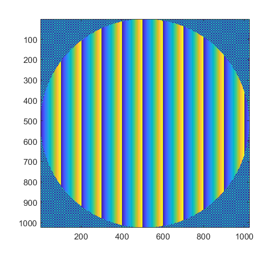
Fig. 23 Example of a pattern generated with the GPU

Creating complex textures

The GPU often has significantly less memory than the main computer. This means that methods like otslm.tools.combine() become memory limited sooner. In order to work around this, it is sometimes possible to implement a version which calculates each pattern, adds it to the total array and re-uses the same memory to calculate the next pattern. The otslm.tools.lensesAndPrisms() function implements the Prisms and Lenses algorithm without needing to generate all the patterns before combining.

xyz = randn(3, num_points);
pattern = otslm.tools.lensesAndPrisms(sz, xyz, 'gpuArray', true);

Using a GeForce GTX 1060 GPU to run the Prisms and Lenses algorithm produces a order of magnitude decrease in run-time for multiple traps compared to a i7-8750H CPU, as shown in Fig. 24.

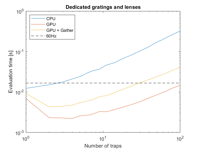
Fig. 24 Comparison of hologram generation time using CPU and GPU with different numbers of traps. For reference, a line is marked corresponding to the 60Hz refresh rate of a moderately fast SLM.

Using iterative algorithms

Iterative algorithms can use GPU arrays if either the target or guess are gpuArrays or if the iterative method is constructed using the named parameter 'gpuArray', true. Not all methods support using the GPU at this stage, for instance, Bowman2017 has not been modified to support the GPU. The iterative methods have not been optimised and they currently involve a lot of copy/matrix resizing operations which will probably slow down optimisation. We aim to address these limitations in future versions.

sz = [512, 512];
im = otslm.simple.aperture(sz, sz(1)/20, 'value', [0, 1], 'gpuArray', true);
gs = otslm.iter.GerchbergSaxton(im, 'adaptive', 1.0, 'objective', []);
pattern = gs.run(600, 'show_progress', false);

Uploading a shader to the GPU

For uploading OpenGL shaders to the GPU, we provide an interface to RedTweezers. RedTweezers operates as a UDP server that runs independently from Matlab, this means it can run on any computer with OpenGL capabilities connected to your network (with appropriate firewall permission). Images, shaders and other data can be sent to RedTweezers via UDP, the RedTweezers server deals with uploading the shader and managing the shaders memory. RedTweezers interfaces are located in otslm.utils.RedTweezers.

Installing RedTweezers

To use RedTweezers, you will need to download the executable and have it running on a computer that is accessible on your network. RedTweezers can be downloaded from the computer physics communications program summaries page. Once downloaded, unzip the file (on windows you can use a program such as 7-zip to extract the files from the .tar.gz archive). Once unzipped, run either the hologram_engine_64.exe (or hologram_engine.exe for the 32-bit version). On the first run you may need to allow access to your network. If everything worked correctly, a new window with the RedTweezers splash screen should be displayed, shown in Fig. 25.

Fig. 25 Red tweezers splash screen.

Displaying a image with RedTweezers

Displaying images isn’t the intended purpose of RedTweezers, however by loading a shader which simply draws a texture to the screen we can implement a ScreenDevice-like interface using RedTweezers. This is implemented by otslm.utils.RedTweezers.Showable. This class inherits from otslm.utils.Showable (in addition to the RedTweezers base class) and provides all the same functionality of a ScreenDevice object. By default the object is configured to connect to UDP port 127.0.0.1:61557 and display an amplitude pattern. We can change the port and pattern type using the optional arguments.

rt = otslm.utils.RedTweezers.Showable('pattern_type', 'phase');
rt.window= [100, 200, 512, 512];   % Window size [x, y, width, height]
rt.show(otslm.simple.linear([200, 200], 20));

The main difference between ScreenDevice and Showable is the size of the pattern and the size/position of the window. ScreenDevice requires the pattern size to match the size of the window. For Showable, the pattern is stretched to fill the window. A further limitation is the maximum packet size RedTweezers supports only allows images of approximately 400x400 pixels (RedTweezers isn’t intended for displaying images).

Using the RedTweezers Prisms and Lenses

otslm.utils.RedTweezers.PrismsAndLenses implements the Prisms and Lenses algorithm described in the RedTweezers paper (and implemented in the LabView code supplied with RedTweezers). To use the Prisms and Lenses implementation, start by creating a new instance of the object and configure the window and any other RedTweezers properties.

rt = otslm.utils.RedTweezers.PrismsAndLenses();
rt.window= [100, 200, 512, 512];   % Window size [x, y, width, height]

Then we need to configure the shader properties. These are not set by default since they may already be set by another program.

rt.focal_length = 4.5e6;       % Focal length [microns]
rt.wavenumber = 2*pi/1.064;    % Wavenumber [1/microns]
rt.size = [10.2e6, 10.2e6];    % SLM size [microns]
rt.centre = [0.5, 0.5];
rt.total_intensity = 0.0;   % 0.0 to disable
rt.blazing = linspace(0.0, 1.0, 32);
rt.zernike = zeros(1, 12);

This should create a blank hologram. To add spots to this hologram use the addSpot() method. For example, to add a spot to diffract light to a particular coordinate in the focal plane, use:

rt.addSpot('position', [60, 54, 7])
rt.addSpot('position', [-20, 10, -3])
rt.addSpot('position', [40, -37, 0])

If we have more than 50 spots we need to send the spot data as a GLSL texture. The class automatically handles this. If we want to always use a texture, we can set

rt.use_texture = true;

Creating custom RedTweezers shaders

To create a custom GLSL shader and load it using RedTweezers simply inherit from the otslm.utils.RedTweezers.RedTweezers class, load the GLSL shader source using the sendShader(), and use sendUniform() and sendTexture() to send data to the shader. For inspiration, look at the Showable and PrismsAndLenses implementations.