utils Package
The otslm.utils package contains functions for controlling,
interacting with and simulating hardware.
Hardware (and simulated hardware) is represented by classes inheriting
from the Showable and Viewable base classes.
Test* devices
are used for simulating non-physical devices, these are used mainly for
testing algorithms. For converting from a [0, 2*pi) phase range to a
device specific lookup table, the LookupTable
class can be used.
This package contains three sub-packages containing
imaging algorithms,
calibration methods and the
RedTweezers interface.
LookupTable
-
class
otslm.utils.LookupTable(phase, value, varargin)¶ Class representing the phase and pixel values of a lookup table.
Lookup tables can be used by Showable devices, otslm.tools.finalize and otslm.tools.colormap.
- Methods
- load – load a human readable lookup table from a file
- save – save a human readable lookup table to a file.
- sorted – Returns a new lookup table sorted by phase
- resample – Re-sampled lookup table at the specified phases
- linearised – New re-sampled lookup with evenly spaced phase values
- valueMinimised – Arrange lookup table so values are ascending
- Properties
- phase – phase values in lookup table [Nx1 matrix]
- value – pixel values in lookup table [NxM matrix]
- range – range of the lookup table (for phase based tables)
See also LookupTable,
otslm.tools.finalize()andShowable-
LookupTable(phase, value, varargin)¶ Construct a new LookupTable instance
- Usage
- lt = LookupTable(phase, value, …)
- Parameters
- phase (numeric) – [Nx1] vector with phase values
- value (numeric) – [NxM] values to map phase too
- Optional named arguments
- range (numeric) – The range of the look up table. This will typically be either 1 or 2*pi depending on if the lookup table is normalized or un-normalized. The actual ranges of phase values may be less or greater than this range.
-
linearised(lt, numpts, varargin)¶ Generates a new lookup table with evenly spaced values
- Usage
- nlt = lt.linearised(numpts, …) generates a resampled lookup table with evenly spaced values.
- Parameters
- numpts (numeric) – number of evenly spaced values.
- Optional named arguments
- range (numeric) – range to re-sample
[min, max]. (default:[min(lt.phase), max(lt.phase)]). - periodic (logical) – specifies if the range is periodic, if so, the end points count as the same point. Default false.
- range (numeric) – range to re-sample
-
static
load(filename, varargin)¶ Load a lookup table from a file
This is useful if you want to use the lookup table in another program. Otherwise, the recommended way to save a lookup table is by using the matlab save function.
- Usage
- lt = LookupTable.load(filename, …) loads the lookup table.
- Parameters
- filename (char) – filename for lookup table to load
- Optional named arguments
- ‘channels’ channels Array of columns numbers in input file 0 correspond to 0 in output. Negative values correspond to columns in reverse order.
- ‘phase’ column Column of input file taken as phase value. If omitted, i.e. [], assumes 0 to 2*pi linear phase range.
- ‘oformat’ format Output format string (default: uint8)
- ‘format’ format Input format handle (default @uint8)
- ‘mask’ mask Mask for input format (default: none)
- ‘morder’ order Array for order of bits in mask length should be 8, (0: zero bit, 1:8 mask bit, other: one bit). 1:8 is normal bit order, 8:-1:1 is reverse order.
- ‘delim’ delim Deliminator in input file
- ‘nheaderlines’ num Number of header lines in file
The number of channels in the output is determined by the length of the channels array. Each element in the channels array determines which column of the input file (starting at 1) is used to generate the channel data. A value of 0 means that this channel is empty.
The format argument specifies the input data type for each column. Data is read, cast to this type, and then the mask is applied. The output value is then calculated as a uint8 from the bits that were masked using the morder argument.
- Example
Load a 16-bit lookup table with values assigned to the first two channels. The input file has two columns, we use the second.
lookup_table = 'LookupTable.txt';
colormap = otslm.utils.LookupTable.load(lookup_table, ...
  'channels', [2, 2, 0], 'phase', [], 'format', @uint16, ...
  'mask', [hex2dec('00ff'), hex2dec('ff00')]);
-
resample(lt, nphase)¶ Generates a new lookup table re-sampled at the specified phases
- Usage
- nlt = lt.resample(nphase) returns a new lookup table re-sampled at the specified phases. Values assigned to new phases correspond to the nearest values in the old table.
- Parameters
- phase (numeric) – new phase values
-
save(lt, filename, varargin)¶ Save the lookup table to a human readable file
This is useful if you want to use the lookup table in another program. Otherwise, the recommended way to save a lookup table is by using the matlab save function.
- Usage
- lt.save(filename, …) saves the lookup table to file.
- Parameters
- filename (char) – filename to save lookup table too.
- Optional named arguments
- header (char) – header lines describing file contents. Default is a message about when the file was generated.
- cols (numeric) – specifies which columns of values will be written.
- format (enum) – type type of lookup table to write. All formats write the phase in the first column. This argument controls what is placed in additional columns. Currently supported types are:
- 8bit – write a single column of 8 bit integers
- 16bit – write a single column of 16 bit integers
- none – don’t write any additional column
- multi – write one column for each value channel
-
sorted(lt)¶ Returns a new lookup table sorted by phase
- Usage
- nlt = lt.sorted()
-
valueMinimised(lt, valueRangeSz)¶ Arranges lookup table so phase values are ascending but attempts to minimise change in linear index between steps.
- Usage
- nlt = lt.valueMinimised(valueRangeSz) requires information about the size of each valueRange dimension (vector).
Todo
document parameters
See also otslm.utils.Showable.valueRangeSize()
imaging
This sub-package contains functions for generating an image of the intensity at the surface of a phase-only SLM in the far-field of the SLM.
To demonstrate how these function work, we can use the
TestFarfield and TestSlm classes.
From examples/imaging.m, the following code demonstrates how
we can image the incident illumination on the device.
Fig. 57 shows the incident illumination
and output from the two imaging methods.
% Setup camera and slm objects
slm = otslm.utils.TestSlm();
slm.incident = otslm.simple.gaussian(slm.size, 100);
cam = otslm.utils.TestFarfield(slm);

% Generate 1-D profile
im = otslm.utils.imaging.scan1d(slm, cam, 'stride', 10, 'width', 10);

% Generate 2-D raster scan
im = otslm.utils.imaging.scan2d(slm, cam, ...
    'stride', [50,50], 'width', [50,50]);
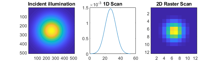
Fig. 57 Example output from imaging functions. (left) incident illumination. (middle) 1-D scan. (right) 2-D raster scan.
scan1d
-
otslm.utils.imaging.scan1d(slm, cam, varargin)¶ Scans a bar region across device.
This function scans a vertical stripe across the surface of the SLM with flat phase. Pixels outside this region are assigned a random phase, a checkerboard pattern or some other pattern in order to scatter light away from the zero order. The camera (or a photo-diode) should be placed in the far-field to capture only light from the flat phase region. This function generates a 1-D profile of the light on the SLM.
- Usage
- im = scan1d(slm, cam, …) scans a bar region across the device and returns a array representing the intensities at each location.
- Parameters
- slm (
Showable) – device to display pattern on. The slm.showComplex function is used to display the pattern. The pattern used for pixels outside the main region depends on the SLM configuration. - cam (
Viewable) – device viewing the display. This device could be a single photo-diode or the average intensity from all pixels on a camera.
- slm (
- Optional named arguments
- width (numeric) – width of the region to scan across the device
- stride (numeric) – number of pixels to step
- padding (numeric) – offset for initial window position
- delay (numeric) – number of seconds to delay after displaying the image on the SLM before imaging (default: [], i.e. none)
- angle (numeric) – direction to scan in (rad)
- angle_deg (numeric) – direction to scan in (deg)
- verbose (logical) – display additional information about run
See also
image2d().
scan2d
-
otslm.utils.imaging.scan2d(slm, cam, varargin)¶ Scans a 2-D region region across device.
This function is similar to
scan1d()except it scans a rectangular region in a raster pattern across the surface of the SLM to form a 2-D image of the intensity.- Usage
- im = scan2d(slm, cam, …) scans a bar region across the device and returns a matrix representing the intensities at each location.
- Parameters
- slm (
Showable) – device to display pattern on. The slm.showComplex function is used to display the pattern. The pattern used for pixels outside the main region depends on the SLM configuration. - cam (
Viewable) – device viewing the display. This device could be a single photo-diode or the average intensity from all pixels on a camera.
- slm (
- Optional named arguments
- width [x,y] (numeric) – width of the region to scan across the device
- stride [x,y] (numeric) – number of pixels to step
- padding [x0 x1 y0 y1] (numeric) – offset for initial window position
- delay (numeric) – number of seconds to delay after displaying the image on the SLM before imaging (default: [], i.e. none)
- angle (numeric) – direction to scan in (rad)
- angle_deg (numeric) – direction to scan in (deg)
- verbose (logical) – display additional information about run
See also
image1d().
calibration
This sub-package contains functions for calibrating the device and generating a lookup-table. Most of these methods assume the SLM and camera are positioned in one of the configurations shown in Fig. 58.
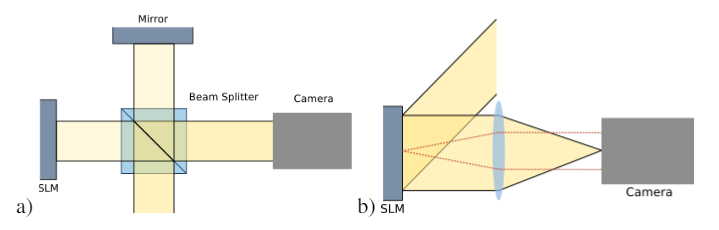
Fig. 58 Two different SLM configurations. (a) shows a Michelson interferometer setup. The SLM and reference mirror will typically be tilted slightly relative to each other. (b) shows a camera imaging the far-field of the device.
The sub-package contains several methods using these configurations.
Some of the methods can be fairly unstable. The most robust methods,
from our experience, are smichelson and step, both are described
below. For information on the other methods, see the file comments and
examples/calibration.m.
smichelson
This setup requires the device to be imaged using a sloped Michelson interferometer. The method applies a phase shift to half of the device and measures the change in fringe position as a function of phase change. The unchanged half of the device is used as a reference.
The easiest way to use this method is via the
otslm.ui.CalibrationSMichelson
graphical user interface.
The method takes two slices through the output image of the Viewable
object. The slices should be perpendicular to the interference fringes
on the SLM. The step width determines how many pixels to average over.
One slice should be in the unshifted region of the SLM, and the other in
the shifted region of the SLM. The slice offset, angle and width
describe the location of the two slices. The step_angle parameter
sets the direction of the phase step.
In order to understand the function parameters, we recommend using the
otslm.ui.CalibrationSMichelson GUI with
the otslm.ui.TestMichelson GUI.
A possible configuration is shown in Fig. 59.
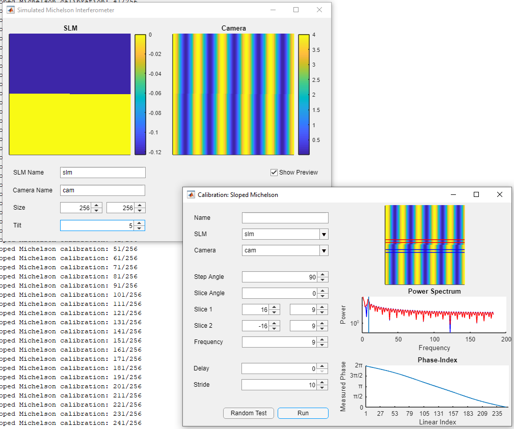
Fig. 59 otslm.ui.CalibrationSMichelson and :
otslm.ui.TestMichelson used to demonstrate the
smichelson calibration method.
-
otslm.utils.calibration.smichelson(slm, cam, varargin)¶ Uses images from a sloped Michelson interferometer
Calculate the SLM lookup table using interference fringes on a sloped Michelson interferometer setup. Either the SLM or reference beam mirror must be sloped with respect to the illumination causing interference fringes in the output. By varying the phase on the device, the fringes can be made to move. This can be done on half the device allowing the other half to be used as a reference.
- Usage
- lt = smichelson(slm, cam, …) calibrate using the smichelson method.
- Parameters
- slm (
Showable) – device to generate the lookup table for. - cam (
Viewable) – device imaging the slm. The camera should be viewing the output of a Michelson interferometer, with the SLM on one arm and a mirror on the other. The mirror should be tilted slightly to create interference fringes on the camera.
- slm (
- Optional named parameters
- slice1_offset num – slice 1 distance from image centre
- slice1_width num – width of the slice 1 to average over
- slice2_offset num – slice 2 distance from image centre
- slice2_width num – width of the slice 2 to average over
- slice_angle num – angle for the slice (deg)
- freq_index idx – index for frequency sample
- step_angle num – angle for the step function (deg)
- delay num – delay after displaying slm image
- stride num – number of linear indexes to step
- basevalue num – value to use for the first region
- verbose bool – display progress in console
- show_progress bool – show progress figure
- show_camera bool – show what the camera sees
- show_spectrum bool – show the 1-D Fourier spectrum of the images
step
This function requires the camera to be in the far-field of the device.
The function applies a step function to the device, causing a
interference line to appear in the far-field. The position of the
interference line changes depending on the relative phase of the two
sides of the step function. An extension to this function is
pinholes() which uses two pinholes instead of a step
function, allowing for more precise calibration.
The easiest way to use this method is via the
CalibrationStepFarfield GUI.
In order to understand the function parameters, we recommend using the
CalibrationStepFarfield GUI with the TestFarfield GUI.
An example configuration is shown in Fig. 60.
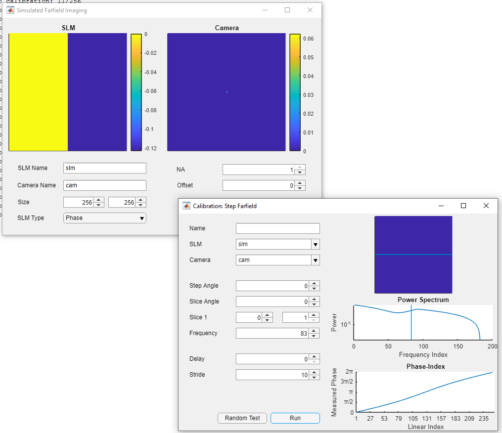
Fig. 60 otslm.ui.CalibrationStepFarfield and :
otslm.ui.TestFarfield used to demonstrate the
step calibration method.
-
otslm.utils.calibration.step(slm, cam, varargin)¶ Applies a step function and looks at interference.
This function creates a step phase pattern with two regions. The far-field interference pattern of these regions contains a fringe which moves depending on the relative phase between the two regions.
The function uses a Fourier transform to determine the position of the interference fringe. The frequency for the Fourier transform is specified by the
freq_indexparameter. The width and angle parameters control the number of pixels to average over and the angle of the slice.- Usage
- lt = step(slm, cam, …) calibrates using the step method.
- Parameters
- slm (
Showable) – device to generate the lookup table for. - cam (
Viewable) – device imaging the slm in the far-field.
- slm (
- Optional named arguments
- slice_offset num – slice distance from image centre
- slice_width num – width of the slice to average over
- slice_angle num – angle for the slice (deg)
- freq_index idx – index for frequency sample
- step_angle num – angle for the step function (deg)
- delay num – delay after displaying slm image
- stride num – number of linear indexes to step
- basevalue num – value to use for the first region
- verbose bool – display progress in console
- show_progress bool – show progress figure
- show_camera bool – show what the camera sees
- show_spectrum bool – show the 1-D Fourier spectrum of the images
pinholes
-
otslm.utils.calibration.pinholes(slm, cam, varargin)¶ Generates virtual pinholes with different phase.
Similar to step but looks at interference of two regions on different parts of the device allowing per-pixel or per-region calibration.
- Usage
- lt = pinholes(slm, cam, …) calibrates using the pinholes method.
- Parameters
- slm (
Showable) – device to generate the lookup table for. - cam (
Viewable) – device imaging the slm in the far-field.
- slm (
- Optional named arguments
- slice_offset num – slice distance from image centre
- slice_width num – width of the slice to average over
- slice_angle num – angle for the slice (deg)
- freq_index idx – index for frequency sample
- delay num – delay after displaying slm image
- stride num – number of linear indexes to step
- basevalue num – value to use for the first region
- radius num – radius of pinholes (pixels)
- verbose (logical) – display progress in console
- show_progress (logical) – show progress figure
- show_camera (logical) – show what the camera sees
- show_spectrum (logical) – show the 1-D Fourier spectrum of the images
checker
-
otslm.utils.calibration.checker(slm, cam, varargin)¶ Generate phase device lookup table using checkerboard pattern.
This method displays a checkerboard pattern on the device and looks at the intensity of the zero-th order. This may not be very effective if the device is not efficient or the device doesn’t cover the full 2*pi phase range.
- Usage
- lt = checker(slm, cam, …)
- Parameters
- slm (
Showable) – device to generate the lookup table for. - cam (
Viewable) – device imaging the slm in the far-field.
- slm (
- Optional named arguments
- spacing (numeric) – size of checkerboard grid
- delay (numeric) – delay after updating slm
- stride (numeric) – number of linear indexes to step
- verbose (logical) – display progress in console
- show_progress (logical) – display progress of the method
- show_camera (logical) – show what the camera sees
linear
-
otslm.utils.calibration.linear(slm, cam, varargin)¶ Attempt to optimise diffraction from a linear grating.
This method does not produce a good estimate of the lookup table but is useful for generating a lookup table to maximise deflection into a particular direction or region.
Warning
This method is experimental.
- Usage
- lt = linear(slm, cam, …)
- Parameters
- slm (
Showable) – device to generate the lookup table for. - cam (
Viewable) – device imaging the slm in the far-field.
- slm (
- Optional named arguments
- grating str – type of grating to display on the device
- max_iterations num – maximum number of iterations to run
- show_progrerss bool – show progress of the method
- method str – method to use for optimisation
- dof num – number of degrees of freedom
- spacing num – diffraction grating spacing
- initial_cond str – initial condition
michelson
-
otslm.utils.calibration.michelson(slm, cam, varargin)¶ Uses images from a standard Michelson interferometer
Requires the SLM to be configured in Michelson interferometer setup where the screen is perpendicular to the incident beam and so is the reference beam mirror.
This method could be extended to allow calibration of individual pixels on the device but requires the uniform illumination.
- Usage
- lt = michelson(slm, cam, …) calibrate the slm using the Michelson interferometer method.
- Parameters
- slm (
Showable) – device to generate the lookup table for. - cam (
Viewable) – device imaging the slm. The camera should be viewing the output of a Michelson interferometer, with the SLM on one arm and a mirror on the other.
- slm (
- Optional named arguments
- delay (numeric) – delay after displaying slm image (seconds).
- stride (numeric) – number of linear indexes to step
- verbose (logical) – display progress in console
RedTweezers
The RedTweezers sub-package provides classes for displaying patterns
using OpenGL using the GPU or OpenGL enabled CPU.
The main class is RedTweezers which provides methods for
setting up the connection to the RedTweezers UDP server and sending
OpenGL uniforms, textures and shaders programs to the UDP server.
For these classes to work, you must have a running RedTweezers
UDP server setup on your network.
For example usage, see the Using the GPU example.
RedTweezers base class
-
class
otslm.utils.RedTweezers.RedTweezers(address, port)¶ Interface to RedTweezers.
RedTweezers is a software package which calculates the hologram using OpenGL and directly displays the hologram on the hardware. This has the advantage over other methods that it does not require the pattern to be downloaded from the graphics hardware and re-uploaded for display on the hardware.
This class connects to RedTweezers via UDP. The RedTweezers library must be running for this to work.
For details and download link, see the RedTweezers CPC paper: https://doi.org/10.1016/j.cpc.2013.08.008
- Methods
- RedTweezers – Construct an instance of this object
- sendCommand – Send a command (adds data block wrapper)
- updateAll – Resend all commands
- readGlslFile – Read a GLSL file into a character array
- Properties
- udp_port – port of RedTweezers server
- live_update – True if property changes should be sent to
RedTweeezers immediately, otherwise
updateAllcan be used to send properties at a later time.
- RedTweezers properties
- vsync (logical) – Synchronise updating with monitor refresh rate
- window (cell|numeric) – Size of the window [x, y, width, height] or
{‘fullscreen’, monitor_id} for fullscreen. Use
resizeWindowto change the window size. - network_reply (logical) – If True, requests RedTweezers server sends a reply.
See also RedTweezers,
ShowableandPrismsAndLenses.-
RedTweezers(address, port)¶ RedTweezers construct a new RedTweezers interface
- Usage
- rt = RedTweezers([address, port]) specifies a custom address/port.
- Parameters
- address – IP address, passed to
udp(). (default: ‘127.0.0.1’). - port – UDP port to connect to (default: 61556).
- address – IP address, passed to
-
static
readGlslFile(filename)¶ Read a GLSL file into a character array
- Usage
- contents = RedTweezers.readGlslFile(filename) Returns a character vector with file contents.
- Parameters
- filename (char) – GLSL file to read
-
sendCommand(rt, cmd)¶ Send a command string to the device
- Usage
- rt.sendCommand(cmd) sends the command string to the device and adds the data block.
- Parameters
- cmd (char) – command string to send to device
-
sendShader(rt, shader, send)¶ Send a shader to the device
- Usage
- cmd = rt.sendShader(shader, [send])
- Parameters
- shader (char) – shader character vector.
- send (logical) – If send is false, the command isn’t sent. (default: nargout == 0)
-
sendTexture(rt, id, texture, varargin)¶ Send a texture blob to the device
- Usage
- cmd = sendTexture(id, texture, [send, …])
- Paramters
- id – OpenGL uniform id to store texture at
- texture – The texture. Should be a 4xWxH in RGBA order. If the texture is a 3xWxH uint8 matrix, the function adds 255 for the A channel.
- send (logical) – If send is false, the command isn’t sent. (default: nargout == 0)
- Optional named arguments
- endian (enum) – ‘L’ or ‘B’ endian-ness of byte stream (for float)
-
sendUniform(rt, id, values, send)¶ Sends an array of namers to the device and renders the pattern
- Usage
- cmd = rt.sendUniform(id, values, [send]) sends an array of numbers. The array of numbers will be stored in uniform register id. The first uniform in the program is id=0. Array length must be less than 200 elements. Returns the string for the command.
- Parameters
- id (numeric) – OpenGL register to store values in
- values (numeric) – array of values to send
- send (logical) – If send is false, the command isn’t sent. (default: nargout == 0)
-
updateAll(rt, send)¶ Resends all information to RedTweezers
Only sends set options (leaves others at RedTweezers defaults)
- Usage
rt.updateAll([send]) send all commands to the device.
cmd = rt.updateAll([send]) send all commands to the device and return the string that is sent.
- Parameters
- send (logical) – If send is False, don’t actually send the commands to the device. (default: nargout == 0)
Showable
-
class
otslm.utils.RedTweezers.Showable(varargin)¶ RedTweezers interface for displaying pre-computed patterns. Inherits from
otslm.utils.ShowableandRedTweezers.Loads a shader into RedTweezers for displaying images. This is roughly equivilant to the ScreenDevice class.
-
Showable(varargin)¶ Connects to RedTweezers and loads the Prisms and Lenses shader
rt = RedTweezers(…) connect to a running instance of RedTweezers. Default address is 127.0.0.1 port 61556.
rt = RedTweezers(address, port, …) specifies a custom address/port.
- Optional named arguments
- ‘lookup_table’ table – Lookup table to use for device Default lookup table is value_range{1} repeated for each channel.
- ‘value_range’ table – Cell array of value ranges Default is 256x3 for a RGB screen
- ‘pattern_type’ str – Type of pattern the device displays. Default is ‘amplitude’. Can also be ‘phase’.
- prescaledPatterns bool – Default value for prescaled argument in show. Default: false.
-
showRaw(rt, img)¶ Show the pattern on the device (update the texture)
rt.showRaw() clears the screen.
rt.showRaw(img) display an image on the screen. The image should have 1 or 3 channels.
Images must be single, double or unit8. Float images should be in range [0, 1), uint8 in range [0, 256).
-
PrismsAndLenses
-
class
otslm.utils.RedTweezers.PrismsAndLenses(varargin)¶ Prisms and Lenses algorithm for RedTweezers. Inherits from
RedTweezers.Implements the Prisms and Lenses algorithm in an OpenGl shader.
See also PrismsAndLenses and
Showable.-
PrismsAndLenses(varargin)¶ Connects to RedTweezers and loads the Prisms and Lenses shader
rt = RedTweezers() connect to a running instance of RedTweezers. Default address is 127.0.0.1 port 61556.
rt = RedTweezers(address, port) specifies a custom address/port.
-
addSpot(rt, varargin)¶ Add a spot to the pattern
rt.addSpot(position, …) declares a new spot at the specified position [x, y, z]. Uses
PrismsAndLensesSpotto represent the spot.- Optional named parameters:
- ‘oam’ int – Vortex charge
- ‘phase’ float – Phase offset for the spot
- ‘intensity’ float – Intensity for the spot
- ‘aperture’ [x, y, R] – Position and radius of aperture
- ‘line’ [x, y, z, phase] – Direction, length and phase of line
-
removeSpot(rt, index)¶ Remove the specified spot from the pattern
rt.removeSpot() removes a spot from the end of the array.
Can also directly modify the Spot array
-
updateAll(rt, send)¶ Resends all information to RedTweezers
Only sends set options (leaves others at RedTweezers defaults) Does not send the shader.
If send is false, the command isn’t sent. Default value for send is nargout == 0
-
PrismsAndLensesSpot
-
class
otslm.utils.RedTweezers.PrismsAndLensesSpot(varargin)¶ Properties definition for a PrismsAndLenses spot. This class is for use with
PrismsAndLenses.- Properties
- position – Position of spot [x; y; z]
- oam – Orbital angular momentum charge number (int)
- phase – Phase of the spot
- intensity – Intensity of the spot
- aperture – Aperture to define hologram within [x; y; radius]
- line – Line trap direction and phase [x; y; z; phase]
-
PrismsAndLensesSpot(varargin)¶ Declares a new spot for PrismsAndLenses
PrismsAndLensesSpot(position, …) declares a new spot at the specified position [x, y, z].
- Optional named parameters
- ‘oam’ int – Vortex charge
- ‘phase’ float – Phase offset for the spot
- ‘intensity’ float – Intensity for the spot
- ‘aperture’ [x, y, R] – Position and radius of aperture
- ‘line’ [x, y, z, phase] – Direction, length and phase of line
Base classes of showable and viewable objects
These abstract base classes define the interface expected by the various imaging, calibration and GUI functions/classes in the toolbox. You can not directly create instances of these classes, instead you must implement your own subclass or use one of the predefined subclasses, see Physical devices or Non-physical devices.
Showable
-
class
otslm.utils.Showable(varargin)¶ Represents devices that can display a pattern. Inherits from
handle.- Methods (abstract):
- showRaw(pattern) – Display the pattern on the device. The pattern is raw values from the device valueRange (i.e. colour mapping should already have been applied).
- Methods:
- show(pattern) – Display the pattern on the device. The pattern type is determined from the patternType property.
- showComplex(pattern) – Display a complex pattern. The default behaviour is to call show after converting the pattern to the patternType of the device. Conversion is done by calling otslm.tools.finalize with for amplitude, phase target.
- showIndexed(pattern) – Display a pattern with integers describing entries in the lookup table.
- view(pattern) – Calculate the raw pattern.
- viewComplex(pattern) – Calculate the raw pattern from complex
- viewIndexed(pattern) – Calculate the raw pattern from indexed
- valueRangeNumel() – Total number of values device can display
- Properties (abstract):
- valueRange – Values that the device patterns can contain. This should be a 1-d array, or cell array of 1-d arrays for each dimension of the raw pattern.
- patternType – Type of pattern, can be one of:
- ‘phase’ – Real pattern in range [0, 1]
- ‘amplitude’ – Real pattern in range [0, 1]
- ‘complex’ – Complex pattern, abs(value) <= 1
- size – Size of the device [rows, columns]
- lookupTable – Lookup table for show -> raw mapping
This is the interface that utility functions which request an image from the experiment/simulation use. For declaring a new display device, you should inherit from this class and define the abstract methods and properties described above. You can also override the other methods if needed.
See also Showable and otslm.utils.ScreenDevice.
-
Showable(varargin)¶ Constructor for Showable objects, provides options for default vals
- Optional named arguments
- prescaledPatterns bool – Default value for prescaled argument in show. Default: false.
-
linearValueRange(varargin)¶ Generate an array of all possible device value combinations
linearValueRange(‘structured’, true) generates a table with as many rows as valueRange has cells.
lienarValueRange() generates a table with a single column. values in each column of valueRange must be column unique.
-
show(varargin)¶ Method to show device type pattern
slm.show(…) with no pattern opens the window with an empty pattern.
slm.show(pattern, …) displays the pattern after applying the color map. For phase based devices, the pattern should not be scalled by 2*pi (i.e. mod(pattern, 1)*2*pi should give the angle).
- Optional named arguments:
- – prescaled bool – If the pattern is already scalled by 2*pi.
- Default: false.
Additional arguments are passed to showRaw.
See also view, showRaw, showComplex.
-
showComplex(pattern, varargin)¶ Default function to display a complex pattern on a device
slm.showComplex(pattern, …) Additional arguments are passed to showRaw.
-
showIndexed(slm, pattern, varargin)¶ Display a pattern described by linear indexes on the device
slm.showIndexed(pattern, …) Additional arguments are passed to showRaw.
-
valueRangeSize(idx)¶ Calculate the size of the lookup table
-
view(slm, pattern)¶ Generate the raw pattern that is displayed on the device
im = slm.view(pattern) apply the modulo (if phase device) and apply the lookup table. Any nans remaining in the image are replaced by the first value in the lookup table.
-
viewComplex(slm, pattern)¶ Convert the complex pattern to a raw pattern
-
viewIndexed(slm, pattern)¶ Convert the indexed pattern to a raw pattern
Viewable
-
class
otslm.utils.Viewable¶ Abstract representation of objects that can be viewed (cameras). Inherits from
handle.- Methods (Abstract)
- view() Show an image from the device.
- Methods
- viewTarget() Show an image of the target region from the device. The default behaviour is just to call view().
- crop(roi) Create a region of interest that is returned by viewTarget. Can have multiple regions.
- Properties (Abstract)
- size Size of the device [rows, columns]
- roisize Size of the target region [rows, columns]
This is the interface that utility functions which request an image from the experiment/simulation use. For declaring a new camera, you should inherit from this class and define the view method.
-
crop(cam, roi)¶ Crop the image to a specified ROI
cam.crop([]) resets the roi to the full screen.
cam.crop(rect) creates a single region of interest described by the rect [xmin ymin width height].
cam.crop({rect1, rect2, …}) creates multiple regions of interest described by separate rects.
-
viewTarget(varargin)¶ View the target, applies a ROI to the result of view()
im = viewTarget(…) acquire one or more target regions and return them to an cell array of images. Specify target regions using the crop function. If no output is requested, the image will be displayed in the current axes.
- Optional named arguments
- roi array Specified which roi to return
See also otslm.Viewable.crop.
Physical devices
These classes are used to interact with hardware, including cameras, screens and photo-diodes.
ScreenDevice
Represents a device controlled by a window on the screen. Devices including some digital micro-mirror devices and spatial light modulators can be connected as additional monitors to the computer and can be controlled by displaying an image on the screen. This class provides an interface for controlling a Matlab figure, making sure the window has the correct size, and ensures the window is positioned above other windows on the screen.
To use the ScreenDevice class, you need to specify which screen to
place the window on and how large the screen should be.
The ScreenDevice can either occupy the whole screen, for example
slm = otslm.utils.ScreenDevice(2, 'pattern_type', 'phase');
would create a full-screen window on display number 2; or the class can create a window of a specified size, for example
slm = otslm.utils.ScreenDevice(1, 'pattern_type', 'amplitude', ...
      'size', [512, 512], 'offset', [100, 100]);
creates a 512x512 window positioned 100 pixels from the bottom and 100 pixels from the left of screen 1. Size must always be positive numbers, while offset can be negative to indicate a position relative to the right/top of the screen, for details, see figure Fig. 61.
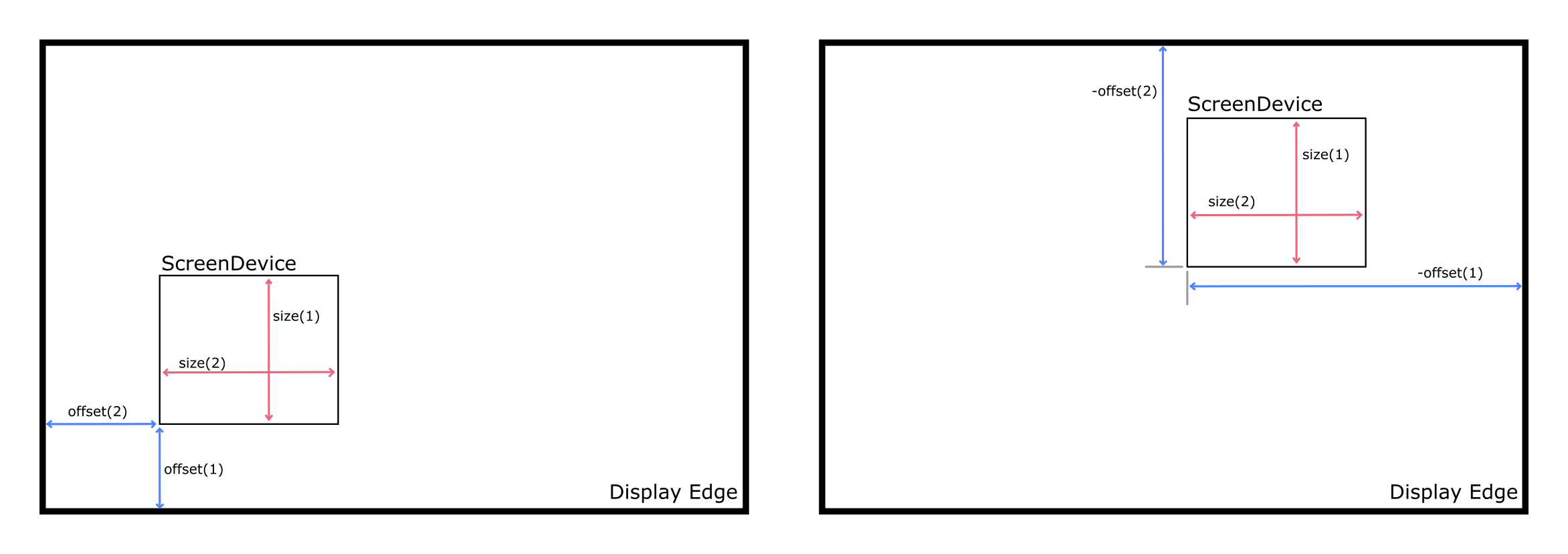
Fig. 61 Position and size of the screen device and display showing how they
relate to the ScreenDevice offset and size input
parameters. (left) a ScreenDevice positioned relative to
the bottom left corner, offset is positive. (right) a
ScreenDevice positioned relative to the top right
corner, offset is negative.
The pattern_type argument specifies if the input pattern to the
show methods should be a phase, amplitude or complex amplitude
pattern. To create a window that is not full-screen, we can simply pass
false as the full-screen argument and set the corresponding target
window size and position offset.
To display a pattern on the device for 10 seconds, we can use
pattern = otslm.simple.linear(slm.size, 50);
slm.show(pattern);
pause(10);
slm.close();
This configuration assumes the pattern has not yet been passed to the
finalize function (i.e. for a linear grating with a spacing of 50
pixels, the pattern should be in the range 0 to 1 and not 0 to 2pi). If
you are using pre-scaled patterns (in the range 0 to 2pi), you can set
the prescaledPatterns optional parameter in the constructor for the
ScreenDevice to true:
slm = otslm.utils.ScreenDevice(scid, 'pattern_type', 'phase', ...
  'prescaledPatterns', true);
To display a sequence of frames on the device, you can use multiple
calls to ScreenDevice.show(). This will apply the colour-map during
the animation, which can be time consuming and reduce the frame rate. An
alternative is to pre-calculate the animation frames. To do this, we
generate a struct which can be passed to the movie function:
% Generate images first
patterns = struct('cdata', {}, 'colormap', {});
for ii = 1:100
  patterns(ii) = im2frame(otslm.tools.finalize(otslm.simple.linear(slm.size, ii), ...
      'colormap', slm.lookupTable));
end

% Then display the animation
slm.showRaw(patterns, 'framerate', 100);
slm.close();
Showable classes have multiple methods for showing patterns on the
device. The showRaw method takes patterns that are already in the
range of values suitable for the device. The show function converts
the specified pattern into the device value range (by applying, for
example, a colour-map or modulo to the pattern). The type of input to
the show function should match the patternType property, for
ScreenDevice objects, patternType is set from the
pattern_type parameter in the constructor. If patternType is
amplitude, the input to show is assumed to be a real amplitude pattern,
if patternType is phase, the input is assumed to be a phase pattern.
The showComplex function uses otslm.tools.finalize() to convert
the complex amplitude to a phase or amplitude pattern (depending on the
value for patternType), before calling show to display the
pattern on the device. Further details can be found in the documentation
for the Showable base class.
To setup the lookup table which is applied by show, we can load a
lookup table from a file and pass it in on construction. If you don’t
yet have a lookup table, you can use one of the calibration functions,
see calibration. As an example, to load a lookup
table specified by a filename fname we could use the following:
lookup_table = otslm.utils.LookupTable.load(fname, ...
  'channels', [2, 2, 0], 'phase', [], 'format', @uint16, ...
  'mask', [hex2dec('00ff'), hex2dec('ff00')], 'morder',  1:8);
This assumes the file has 2 columns, we ignore the first and split the
second into the lower 8 bits and upper 8 bits. The lookup table has 3
channels, the first two channels have values from the second column in
the file, the third channel is all zeros. The format for the input is
uint16, we apply a mask to this input for each column and we
specify the order of the bits from least significant to most significant
(morder). The phase isn’t specified in this lookup table, so we
assume it is linear from 0 to 2pi. For further details, see
LookupTable.
To use this lookup table for the ScreenDevice, we simply pass it
into the constructor:
slm = otslm.utils.ScreenDevice(1, ...
    'lookup_table', lookup_table, ...
    'pattern_type', 'phase');
-
class
otslm.utils.ScreenDevice(varargin)¶ Represents a device controlled by a window on the screen Inherits from
Showable.Useful for displaying images on SLMs and DMDs connected as a screen on the computer running Matlab.
The actual target device size may be smaller than the size reported by the device.
See also ScreenDevice, show, otslm.utils.Showable.
-
ScreenDevice(varargin)¶ ScreenDevice Construct a new instance of the screen device.
screen = ScreenDeivce(device_number, …) creates a new screen device for the specified physical device. Patterns are assumed to be amplitude based, value range is RGB.
- Optional named parameters:
- ‘size’ [r,c] – Size of the device within the window Default: [], (i.e. slm.device_size)
- ‘offset’ [r,c] – Offset within the window. Negative values are offset from the top of the screen. Default: [0, 0]
- ‘lookup_table’ table – Lookup table to use for device Default lookup table is value_range{1} repeated for each channel.
- ‘value_range’ table – Cell array of value ranges Default is 256x3 for a RGB screen
- ‘pattern_type’ type – Type of pattern the device displays. Default is amplitude.
- ‘fullscreen’ bool – Default value for showRaw/fullscreen
- ‘prescaledPatterns’ bool If the pattern is already pre-scaled.
-
close()¶ Close the window used to control the device
-
showRaw(varargin)¶ Show the window and (optionally) display an image
showRaw() display a blank screen.
showRaw(img) display an image on the screen. The image should have 1 or 3 channels.
showRaw(frames) displays frames using the movie command. frames should be an array of frames generated by im2frame. showRaw(frame, ‘framerate’, rate) specifies the frame rate. showRaw(frame, ‘play’, times) specifies time to play (see movie).
-
GigeCamera
Showable wrapper for cameras using the gigecam interface. This
class uses the snapshot function to get an image from the device.
The gigecam device is stored in the device property of the
class.
-
class
otslm.utils.GigeCamera(varargin)¶ Connect to a gige camera connected to the computer Inherits from
Viewable.- Properties
- device – gige camera object
- size – size of the camera output image
- Exposure – camera exposure setting
See also GigeCamera
-
GigeCamera(varargin)¶ Connect to the camera
cam = GigeCamera(device_id) connects to the specified GIGE camera. device_id is passed to the gigecam function.
WebcamCamera
Showable wrapper for windows web-cameras. Uses the
videoinput('winvideo', ...) function to connect to the device. This
class uses the getsnapshot function to get an image from the device.
The videoinput device is stored in the device property of the
class.
Note
This class currently doesn’t inherit from ImaqCamera
but is likely to in a future release of OTSLM.
-
class
otslm.utils.WebcamCamera(varargin)¶ Connect to a webcam camera connected to the computer. Inherits from
Viewable.- Properties
- size – resolution of the device
- device – videoinput device for the camera
This call can be used to create a otslm.utils.Viewable instance for a videoinput source. This requires the Image Acquisition Toolbox.
See also WebcamCamera,
GigeCameraandImaqCamera.-
WebcamCamera(varargin)¶ Connect to the camera
cam = WebcamCamera(device_id) connect to the specified webcam camera. For the device id, imaqhwinfo.
If the device you are interested in is not listed, try resetting/clearing all devices with imaqreset.
ImaqCamera
Showable wrapper for image acquisition toolbox cameras. Uses the
videoinput(...) function to connect to the device. This class uses
the getsnapshot function to get an image from the device. The
videoinput device is stored in the device property of the class.
-
class
otslm.utils.ImaqCamera(varargin)¶ Connect to a image acquisition toolbox (imaq) camera Inherits from
ViewableThis call can be used to create a otslm.utils.Viewable instance for a videoinput source. This requires the Image Acquisition Toolbox.
- Properties
- device – imaq object for the camera
See also ImaqCamera.
-
ImaqCamera(varargin)¶ Connect to the camera
cam = ImaqCamera(adaptor, id, …) conntect to the specified webcam camera. For the device id, imaqhwinfo.
For cameras that support multiple formats, a ‘format’ named argument can be supplied with the format to use.
Non-physical devices
The utils package defines several non-physical devices which can be
used to test calibration or imaging algorithms.
The TestDmd and TestSlm classes are
Showable devices which can be combined with the
TestFarfield or
TestMichelson Viewable devices. These Showable
devices implement the same functions as their physical counter-parts,
except they store their output to a pattern property. The
Viewable devices require a valid TestShowable
instance and implement a view
function which retrieves the pattern property from the
Showable and simulates the expected output.
For example usage, see the examples in the imaging section.
TestDmd
-
class
otslm.utils.TestDmd(varargin)¶ Non-physical dmd-like device for testing code. Inherits from
TestShowable.This class can be used as a non-physical Showable device in simulating a binary amplitude device, such as a digital micro-mirror device.
When
showRawis called, the function calculates the pattern, optionally by applyingrpackusing theotslm.tools.finalize()method, and sets thepatternproperty with the computed pattern. The incident illumination is added to the output. To change the incident illumination, either set a different pattern on construction or change the property value.- Properties
- incident (complex) – incident illumination profile. Must be the same size as the device.
- pattern (comples) – pattern generated by the
showRawmethod. This pattern is is the complex amplitude after multiplying by the incident illumination and applyingrpack. Therpackoperation means that this pattern is larger than the device, with extra padding added to the corners. - use_rpack (logical) – True if
rpackshould be used.
- Constant properties
- size (size) – device resolution (pixels) [rows, columns]
- valueRange – range of raw device values (fixed:
{[0, 1]}) - patternType – type of pattern for device (fixed:
'amplitude') - lookupTable – mapping between gray-scale and binary values. (fixed)
See also TestDmd,
TestSlmandTestFarfield.-
TestDmd(varargin)¶ Create a new virtual DMD object for testing
- Usage
- slm = TestDmd(…) create a virtual binary amplitude device.
- Optional named arguments
- size [row, col] – Size of the device (default: [512,512])
- incident im – Incident illumination (default: [])
- use_rpack (logical) – If
rpackshould be used.
TestSlm
-
class
otslm.utils.TestSlm(varargin)¶ Non-physical slm-like device for testing code. Inherits from
TestShowable.The
showRawfunction applies the inverse of the lookup table, converts from phase to a complex amplitude and assigns the result to thepatternproperty.- Properties
- pattern (complex) – pattern generated by the
showRawmethod. This pattern is the complex amplitude after multiplying by the incident illumination and is the same size as the device. - incident (complex) – incident illumination.
- pattern (complex) – pattern generated by the
- Constant properties
- size (size) – device resolution in pixels [rows, columns]
- valueRange – range of raw device values (default:
{0:255}) - patternType – type of pattern for device (fixed:
'phase') - lookupTable – Lookup table for the device. Defaults to a linear mapping of 0 to 2pi to the discrete colour levels of the device.
See also TestSlm,
TestDmdandTestFarfield.-
TestSlm(varargin)¶ Create a new virtual SLM object for testing
- Usage
- slm = TestSlm(…) creates a device with a linear phase lookup table from 0 to 2*pi.
- Optional named arguments
- size (size) – size of the device (
[rows, cols]). - incident (complex) – incident illumination
- lookup_table – lookup table for colormap
- value_range (cell) – cell array with channel values for raw
pattern. Default:
{0:255}. Use{0:255, 0:255, 0:255}for three channel device with 256 levels on each channel.
- size (size) – size of the device (
TestFarfield
-
class
otslm.utils.TestFarfield(varargin)¶ Non-physical camera for viewing TestShowable objects Inherits from
Viewable.Calculates the paraxial far-field of the
TestShowableobject. The view method callsotslm.tools.visualise()and calculates the intensity of the resulting image (abs(U)^2).Note
This class may change in future versions to use a propagator instead of
otslm.tools.visualise().- Properties
- size – size of the output image
- showable – the Showable object that this class is linked to
- NA – numerical aperture of the lens
(passed to
otslm.tools.visualise()). - offset – offset from the focal plane of the lens
(passed to
otslm.tools.visualise()).
- Inherited properties
- roisize – (Viewable) size of the regions of interest
- roioffset – (Viewable) offsets for the regions of interest
- numroi – (Viewable) number of regions of interest
See also TestFarfield,
TestMichelson,TestSlm.-
TestFarfield(varargin)¶ Construct a new TestFarfield looking at a TestShowable object
- Usage
- obj = TestFarfield(showable, …)
- Parameters
- showable (
TestShowable) – linked showable device.
- showable (
- Optional named arguments
- NA (numeric) – Numerical aperture of lens (default: 1.0)
- offset (numeric) – Offset from focal plane of lens (default: 0.0)
TestMichelson
-
class
otslm.utils.TestMichelson(showable, varargin)¶ Non-physical representation of Michelson interferometer. Inherits from
Viewable.The interferometer consists of two arms, a reference arm with a mirror and a device arm with a
Showabledevice such as a SLM or DMD The TestMichelson simulates aTestShowabledevice placed in one arm, and calculates the interference pattern between the reference arm and the test arm.The
viewfunction gets the currentpatternfrom theTestShowabledevice and calculates the interference. The device supports adding a tilt between the reference arm and the Showable arm. This can be useful for testingcalibration.smichelson().- Properties
- tilt – Angle to tilt the showable device with respect to the reference beam. Applies a exp(2*pi*i*linear*tilt) grating.
- Properties (read-only)
- size – Size of the output image (same as Showable)
- showable – The TestShowable device
See also TestMichelson,
TestShowableandTestFarfield.-
TestMichelson(showable, varargin)¶ Create the new interferometer-like device
- Usage
- obj = TestMichelson(showable, …) construct a new Michelson interferometer to view the TestShowable device.
- Parameters
- showable (
TestShowable) – the device to link
- showable (
- Optional named arguments
- tilt (numeric) – tilt factor (default: 0.0)
TestShowable
-
class
otslm.utils.TestShowable¶ Non-physical showable device for testing implementation. Inherits from
Showable.This is an abstract class defining a single abstract property,
pattern, containing the pattern currently displayed on the device. For implementations seeTestDmdandTestSlm.- Properties (Abstract)
- pattern – complex valued pattern currently displayed on the device.