Getting Started
This page will guide you through getting started with OTSLM. This page is split into three sections: installation, using the GUIs, and writing functions with the toolbox.
Installation
To run OTSLM you need to download the toolbox files and have a
recent version of Matlab installed (we tested OTSLM with Matlab 2018a).
There are a couple of ways to get OTSLM. You can download one of the
Matlab toolbox files (with the .mltbx extension), you can download
a .zip archive containing the source code,
or you can clone the GitHub repository.
The advantage of cloning the GitHub repository is you can easily switch
between different versions of the toolbox or download the most recent
changes/improvements to the toolbox.
There are a range of online tutorials for getting started with
git and GitHub, for example
https://product.hubspot.com/blog/git-and-github-tutorial-for-beginners.
Installing via Matlab Addons Explorer
If using Matlab, the easiest method to install the toolbox is using the Matlab Addons explorer. Simply launch Matlab and navigate to Home > Addons > Get-Addons and search for “OTSLM”. Then, simply click the Add from GitHub button to automatically download the package and add it to the path. You may need to logging to a Mathworks account to complete this step.
Using a .mltbx file
You can download the latest stable release of OTSLM from either the
GitHub release page.
Simply download the appropriate .mltbx file for the relevant version.
Once downloaded, execute the file and follow the instructions to install
the toolbox.
To change/remove the toolbox, go to Home > Add-ons > Manage Add-ons and select the toolbox you would like to configure.
Using a .zip or cloning the repository
The latest version of OTSLM can be downloaded from the
OTSLM GitHub page.
Simply click the Clone or Download button and select your
preferred method of download.
If you are cloning the repository you can checkout different
tags to select the desired release.
Alternatively, for a specific version, navigate to the
release page
and select the .zip file for the desired release.
To install OTSLM, download the latest version of the toolbox to your
computer, if you downloaded a .zip file, extract the files to
your computer.
Once downloaded, most of the toolbox functionality is ready to use. To
start exploring the functionality of the toolbox immediately, you can
run the examples or launch one of the GUIs in the +otslm/+ui
directory. However, for writing your own code, you will probably want to
add the toolbox to the Matlab path. To do this, simply run
addpath('/path/to/toolbox/otslm');
Replace the path with the path you placed the downloaded toolbox in. The
folder must contain the +otslm directory and the docs directory.
If you downloaded the latest toolbox from GitHub, the final part of the
pathname will either be the repository path (if you used git clone)
or something like otslm-master (if you downloaded a ZIP). The above
line can be added to the start of each of your files or for a more
permanent solution you can add it to the Matlab startup
script.
Post installation
To check that otslm was found, run the following command and verify
it displays the contents of the +otslm/Contents.m file
help otslm
If you have multiple versions of otslm downloaded, you may want to
check which version is currently being used.
The following command can be used to check which toolbox
is being used
what otslm
OTSLM is implemented as a Matlab package, all the core functionality is
contained within the +otslm directory and can be accessed by adding
the folder containing +otslm to the path and prefixing the contained
functions with otslm..
For example, to access the linear function in
the simple sub-package, you would use
im = otslm.simple.linear([10, 10], 3);
Some functionality requires additional components. You can choose to install these now or later.
- Optical Tweezers Toolbox (1.5.1 or newer)
- Python (2.7 or newer)
- numpy (tested on 1.13.3)
- theano (tested on 0.9)
- scipy (tested on 1.0)
- pyfftw (optional, for Fourier transform)
- Red Tweezers
- Specific Matlab toolboxes:
- Optimization Toolbox
- Signal Processing Toolbox
- Neural Network Toolbox
- Symbolic Math Toolbox
- Image Processing Toolbox
- Instrument Control Toolbox
- Parallel Computing Toolbox
- Image Acquisition Toolbox
- Matlab MEX compatible C++ compiler
In some cases it is possible to re-write functions to avoid using specific Matlab toolboxes. If you encounter difficultly using a function because of a missing Matlab toolbox, let us know and we may be able to help.
Exploring the toolbox with the GUI
The toolbox includes a graphical user interface (GUI) for many of the
core functions. The user interface allows you to explore the
functionality of the toolbox without writing a single line of code.
The GUIs can be accessed by running the OTSLM Launcher application.
The launcher can be found in the Apps menu (if OTSLM was installed
using a .mltbx file), or run from the file explorer by navigating
to the +otslm/+ui directory and running Launcher.mlapp.
If you have already added OTSLM to the path, you can also start the
launcher by running the following command in the command window
otslm.ui.Launcher
If everything is installed correctly, the launcher should appear, as depicted in Fig. 1. The window is split into 4 sections: a description of the toolbox, a list of GUI categories, a list of applications, and a description about the selected application. Once you select an application, click Launch.
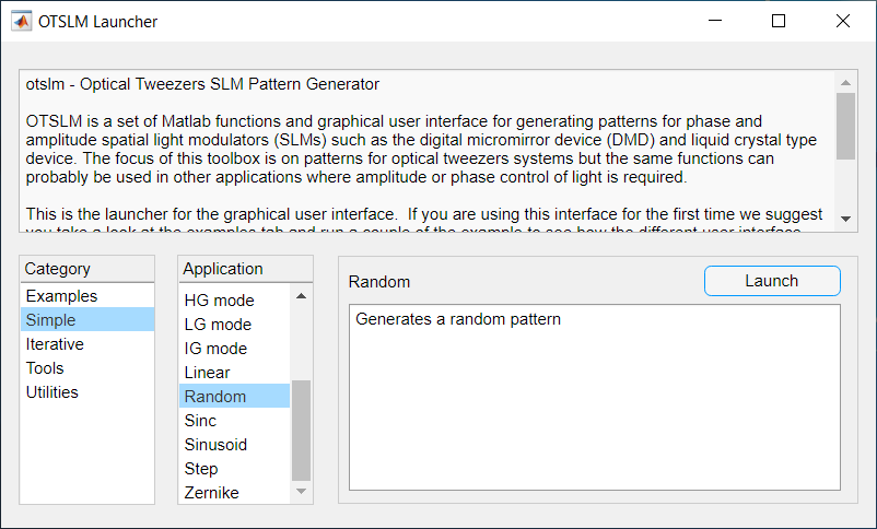
Fig. 1 Overview of the Launcher application.
The output from various applications can either be saved to the Matlab
workspace or sent to a otslm.utils.Showable device
(if one has already been configured).
Applications which generate a pattern have an option to enter a Matlab
variable name. When the pattern is generated, the image is saved to the
current Matlab workspace. Applications which take patterns as inputs (for
example, combine and finalize) can use the patterns produced by another
window by simply specifying the same variable name, for example
see Fig. 2.
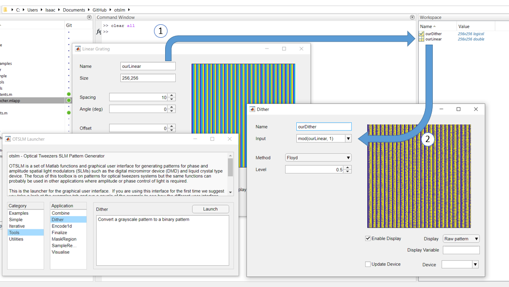
Fig. 2 Illustration showing dataflow between the GUI windows.
A linear grating is generated with the name outLinear,
when the pattern is ready it is saved to the Matlab workspace (1).
This pattern can then be used by other interfaces, for example
(2) shows the same variable name being used as an input to the
Dither application.
If an app produces an error or warning, these will be displayed in the Matlab console.
The example applications show how the user interfaces can be combined to achieve a particular goal. To get started using the GUI, work through these examples. For additional information, see the ui Package documentation.
It is possible to customize these interfaces, however creating custom user interfaces in Matlab is rather time consuming and involves a lot of code duplication. Instead, we recommend using live scripts, see the Gratings and Lens LiveScript example. It is also possible to create a graphical user interfaces in LabVIEW, for details see Accessing OTSLM from LabVIEW.
Using the toolbox functions
The toolbox functions and classes are organised into four main packages:
simple Package, iter Package, tools Package
and utils Package. To use these functions, either prefix the function
with otslm and the package name
im = otslm.simple.linear([10, 10], 3);
import a specific function
import otslm.simple.linear;
im = linear([10, 10], 3);
or import the entire package
import otslm.simple.*;
im1 = linear([10, 10], 3);
im2 = spherical([10, 10], 3);
Most of the toolbox functions produce/operate on 2-D matrices. The type
of values in these matrices depends on the method, but values will
typically be logical, double or complex. Complex matrices are typically
used when the complex amplitude of the light field needs to be
represented. Double matrices are used for both amplitude and phase
patterns. Logicals are returned when the function could be used as a
mask, for instance, otslm.simple.aperture() returns a
logical array by default.
For phase patterns, there are three type of value ranges: [0, 1),
[0, 2*pi) and device specific colour range (after applying a lookup
table to the pattern). Most of the otslm.simple functions return
phase patterns between 0 and 1 or patterns which can be converted to
this range using mod(pattern, 1). To convert these patterns to the
[0, 2*pi) range or apply a specific colour-map, you can use the
otslm.tools.finalize() function.
To get started using the toolbox functions for beam shaping, take a look
at the Beams and Advanced Beams examples.
The examples directory provides examples of other toolbox
functions and how they can be used.
To get help on toolbox functions or classes, type help followed by
the OTSLM package, function, class or method name. For example, to get help
on the otslm.simple package, type:
help otslm.simple
or to get help on the run method in the otslm.iter.DirectSearch
class use
help otslm.iter.DirectSearch/run
For more extensive help, refer to this documentation.