Functions

combine

otslm.tools.combine(inputs, varargin)

Combines multiple patterns

Typical input should be a pattern between 0 and 1. Most methods output range is between 0 and 1.

For iterative combination methods, see otslm.iter.IterCombine or generate a target field using the farfield method and use an otslm.iter.IterBase iterative method.

Usage

pattern = combine(inputs, …) combines the cell array of patterns.

Parameters

• inputs (cell) – cell array of input images to combine. These images should all be the same size.

Optional named parameters

• ‘method’ (enum) – Method to use when combining patterns.

  Methods to create multiple beams

  • dither – Randomly chooses values from different patterns
  • super – Uses phi = angle(sum_ii exp(1i*2*pi*inputs(ii)))
  • rsuper – Superposition with random offset for each layer

  Methods to modulate a beam pattern

  • add – Adds the patterns: sum_ii inputs(ii)
  • multiply – Multiplies the patterns: prod_ii inputs(ii)
  • addangle – Uses phi = angle(prod_ii exp(1i*2*pi*inputs(ii)))
  • average – Weighted average of inputs. (default weights: ones) \(\sum_i w_i I_i / \sum_i w_i\)

  Miscelanious

  • farfield – Calculate farfield sum: sum_ii Prop(inputs(ii)). This method assumes the input has the currect range for the propagator. The default propagator is a FFT, so the inputs should be complex amplitudes.

  Default method: super.

• ‘weights’ (numeric) – Array of weights, one for each pattern. (default: [], uses equal weights for each pattern)

• ‘vismethod’ (fcn) – Used by farfield method. Default: @otslm.tools.prop.FftForward.simpleProp.evaluate.

See also Di Leonardo, Ianni and Ruocco (2007).

dither

The dither() function can be used to convert a continuous gray-scale image into a binary pattern. This can be useful for converting gray-scale amplitude images into binary images for display on a digital micro-mirror device.

The function supports a range of different dither methods including Matlab’s builtin dither, raw thresholding, random dithering and using the Floyd-Steinberg algorithm. The following code example demonstrates a couple of different methods, the results are shown in Fig. 54.

im = otslm.simple.linear([256, 256], 256);
d1 = otslm.tools.dither(im, 0.5, 'method', 'threshold');
d2 = otslm.tools.dither(im, 0.5, 'method', 'mdither');
d3 = otslm.tools.dither(im, 0.5, 'method', 'floyd');
d4 = otslm.tools.dither(im, 0.5, 'method', 'random');

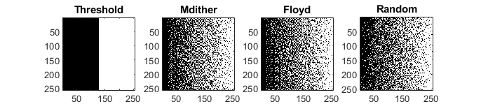
Fig. 54 Example output from dither() using different methods.

otslm.tools.dither(pattern, level, varargin)

Creates a binary pattern from gray-scale image. Supports several different dithering methods.

Usage

pattern = dither(pattern, level, …) applies the default dithering, binary threshold, to the pattern.

Parameters

• pattern (numeric) – the gray-scale pattern. Most methods assume the pattern has values in the range 0 to 1.
• level (numeric) – threshold level

Optional named parameters

• ‘method’ (enum) – Method to use for dithering. Supported methods:

• ‘threshold’ – Apply threshold filter to image (default)
• ‘mdither’ – Use matlab dither function
• ‘floyd’ – Floyd-Steinberg algorithm
• ‘random’ – Does random dithering

• ‘value’ [min, max] Value range for output image (default: [] for logical images). See castValue().

encode1d

otslm.tools.encode1d(target, varargin)

Encode the target pattern amplitude into the phase pattern size

Usage

[pattern, assigned] = encode1d(target, …) encodes the complex target pattern into a 1-D phase mask. Returns the encoded pattern and a logical matrix of the same size that specifies if pixels were used to encode the pattern.

Parameters

• target (numeric) – vector containing values of 1-D amplitude function to be encoded.

Optional named arguments

• ‘scale’ (numeric) – Scale for the height of the pattern
• ‘angle’ (numeric) – Rotation angle about axis (radians)
• ‘angle_deg’ (numeric) – Rotation angle about axis (degrees)

finalize

otslm.tools.finalize(pattern, varargin)

Finalize a pattern, applying a color map and taking the modulo.

Usage

pattern = finalize(input, …) finalizes the pattern. For dmd type devices, the input is assumed to be the amplitude. For slm type devices, the input is assumed to be the phase.

pattern = finalize(phase, ‘amplitude’, amplitude’, …) attempts to generate a pattern encoding both the phase and amplitude.

Parameters

• pattern (numeric) – phase pattern to be finalized

Optional named parameters

• ‘modulo’ (numeric|enum) – Applies modulo to the pattern. Modulo should either be a scalar or ‘none’ for no modulo. (default: 1.0 for slm type devices and ‘none’ for dmd type devices).
• ‘colormap’ – Colormap to apply to pattern. For a list of valid values, see colormap(). (default: ‘pmpi’ for slm and ‘gray’ for dmd type devices).
• ‘rpack’ (enum) – rotation packing of the pixels.

• ‘none’ – No additional steps required (default slm)
• ‘45deg’ – Device is rotated 45 degrees (aspect 1:2, default dmd)

• ‘device’ (enum) – Specifies the type of device, changes the default value for most arguments. If all arguments are provided, this argument has no impact.

• ‘dmd’ – Digital micro mirror (amplitude) device
• ‘slm’ – Spatial light modulator (phase) device

• ‘encodemethod’ method Method to use when encoding phase/amplitude

• ‘checker’ – (default) use checkerboard pattern and acos correction (phase)
• ‘grating’ – Use linear grating and sinc correction (phase)
• ‘magnitude’ – Use grating magnitude modulation (phase)

• ‘amplitude’ pattern Amplitude pattern to generate output for

hologram2volume

otslm.tools.hologram2volume(hologram, varargin)

Generate 3-D volume representation from hologram.

This function is only the inverse of volume2hologram when interpolation is disabled for both.

Usage

volume = hologram2volume(hologram, …) generates a 3-D volume for 2-D complex amplitude hologram. Unwraps hologram onto Ewald sphere.

Parameters

hologram (numeric) – 2-D hologram to map to Ewald sphere.

Optional named arguments

• ‘interpolate’ (logical) – Interpolate between the nearest two pixels in the z-direction. (default: True)
• ‘padding’ (numeric) – Padding in the axial direction (default 0).
• ‘focal_length’ (numeric) – focal length in pixels (default: min(size)/2).
• ‘zsize’ (size) – size for z depth (default: []) The total z size is zsize + 2*padding.

See also volume2hologram() and prop.FftEwaldForward

mask_regions

otslm.tools.mask_regions(base, patterns, locations, sizes, varargin)

Adds patterns to base using masking

Usage

pattern = mask_region(base, patterns, locations, sizes, …)

Parameters

• base (numeric) – base pattern to mask and add regions to
• patterns (cell) – cell array of patterns to be added. Each pattern must be the same size as base. Patterns should be numeric.
• locations (cell) – cell array containing vectors for the centre of each mask region. Must be the same length as patterns.
• sizes – size parameters for each shape (see options below). Number of sizes must be 1 (for a single shape) or match the length of patterns.

Optional named parameters

• ‘shape’ (cell|enum) – shape to use for masking. Must either be a single shape or a cell array of shapes with the same number of elements as patterns. Supported shapes and [sizes] include:

• ‘circle’ [radius] Use a circular aperture.
• ‘square’ [width] Square with equal sides.
• ‘rect’ [w, h] Rectangle with width and height.

sample_region

otslm.tools.sample_region(sz, locations, detectors, varargin)

Generates a pattern for sampling regions on SLM.

Usage

pattern = sample_region(sz, locations, detectors, …) generates the patterns for sampling regions at different SLM locations onto detectors located at detector locations. The range for the pattern is 0 to 1, so the output should be passed to otslm.tools.finalize.

Parameters

• sz (size) – size of the generated pattern [rows, cols]
• locations (cell{numeric}) – cell array of locations in the generated pattern to place regions. {[x1, y1], [x2, y2], ...}. Location shave units of pixels.
• detectors (cell{numeric}) – cell array of numbers describing the locations in the far-field. {[x1, y1], [x2, y2], ...}. This locations are passed into otslm.simple.linear() as the spacing argument. Must be the same length as locations or be a single location. If detectors is a single location, all the patterns will point to the same detector.

Most optional named parameters can also be cell arrays (or cell arrays of cell arrays) for different options for each location.

Optional named parameters

• radii (numeric) – Radius of each SLM region. Should be a single element or an array the same length as locations.
• amplitude (enum) – Specifies a method for amplitude modulation. See below for a list of methods and arguments.
• ampliutdeargs (cell) – Cell array of arguments to pass to amplitude method.
• background (enum) – Specifies the background type. Possible values are:

• ‘zero’ – Uses 0 phase as the background.
• ‘nan’ – Uses NaN phase as the background.
• ‘checkerboard’ – Uses a checkerboard for the background.
• ‘random’ – Uses noise for the background.
• ‘randombin’ – Uses binary noise for the background.

Possible amplitude methods are

• ‘step’ – Sharp step between background and pattern. No parameters.
• ‘gaussian_dither’ – Randomly mixes in background. Parameters:

• ‘offset’ (numeric) – offset for dither threshold.
• ‘noise’ (numeric) – scale of uniform noise to add to pattern.

• ‘gaussian_noise’ – Adds noise to edge of the pattern. Parameters:

• ‘offset’ (numeric) – Offset.
• ‘scale’ (numeric) – Uniform noise range or Gaussian width.
• ‘type’ (enum) – type of noise, either ‘uniform’ or ‘gaussian’

• ‘gaussian_scale’ – Scales the pattern by a Gaussian and then uses the mix method to combine the pattern with the background. The mix method must be ‘add’ for adding the result to the background, or ‘step’ for placing the scaled pattern on the background as a step. Parameters:
• ‘mix’ (enum) – mix method, ‘add’ or ‘step’
• ‘mixargs’ (cell) – arguments for mix method
• ‘scale’ (numeric) – scaling factor

spatial_filter

otslm.tools.spatial_filter(input, filter, varargin)

Applies a spatial filter to the image spectrum. This can be used to simulate imaging or focussing of light using an objective with different shaped apertures or for adding spherical aberration to the system.

Usage

[output, filtered] = spatial_filter(input, filter, …) Applies filter to the Fourier transform of input and calculates the inverse Fourier transform to give output. Optional output filtered is the filtered pattern.

Parameters

• input (numeric) – image to apply filter to.
• filter (numeric) – a mask pattern to apply to the far-field of the input. Should be the same size or smaller than the output of the forward propagation method. If it is smaller, the array is padded with zeros.

Optional named parameters

• vismethod (fcn) – Function to calculate far-field. Takes one argument, the complex amplitude near-field. Default: @otslm.tools.prop.FftForward.simpleProp.evaluate
• invmethod (fcn) – Function to calculate near-field. Takes one argument: the complex amplitude far-field. Default: @otslm.tools.prop.FftInverse.simpleProp.evaluate
• gpuArray (logical) – If the result should be a gpuArray. Default: isa(input, 'gpuarray').

Padding can be controlled by changing the vis and inv methods.

See also examples.liveScripts.booth1998

visualise

otslm.tools.visualise(phase, varargin)

Generates far-field plane images of the phase pattern

Usage

[output, …] = visualise(phase, …) visualise the phase plane. Some methods output additional parameters, such as the ott-toolbox beam.

If phase is an empty array and one of the other images is supplied, the phase is assumed to be an array of zeros the same size as one of the other images.

[output, …] = visualise(complex_amplitude, …) visualise the field with complex amplitude.

Parameters

• phase (real) – The phase image should be in a range from 0 to 2*pi. If the range is approximately 1 a warning is issued.
• complex_amplitude (complex) – a complex amplitude pattern to visualise.

Optional named parameters

• ‘method’ (enum) – Method to use when calculating visualisation. Current supported methods:

• ‘fft’ Use fourier transform approach described in https://doi.org/10.1364/JOSAA.15.000857
• ‘fft3’ Use 3-D Fourier transform, if original image is 2-D, converts to volume and takes Fourier transform. If input is 3-D, directly applies 3-D Fourier transform.
• ‘ott’ Use optical tweezers toolbox (OTT).
• ‘rs’ Rayleigh-Sommerfeld diffraction formula
• ‘rslens’ Use rs to propagate to a lens, apply the lens phase pattern and propagate some distance from the lens.

• ‘type’ type Type of transformation: ‘nearfield’ or ‘farfield’
• ‘amplitude’ image Specifies the amplitude pattern
• ‘incident’ image Specifies the incident illumination Default illumination is uniform intensity and phase.
• ‘z’ z z-position of output plane. For fft/ott this is an offset from the focal plane. For rs/rslens, this is the distance along the beam axis.
• ‘padding’ p Add padding to the outside of the image. Default: ceil(size(phase)/2)
• trim_padding (logical) – Trim padding before returning result (default: false).
• NA (numeric) – Numerical aparture of the lens (default: 0.1)
• resample (numeric) – Number of samples per each pixel (default: []).

bsc2hologram

otslm.tools.bsc2hologram(sz, beam, varargin)

Calculates the far-field hologram for a BSC beam

Requires the optical tweezers toolbox (OTT).

Warning

The current version of the optical tweezers toolbox may introduce additional phase artifacts in the far-field.

Usage

[phase, cpattern] = bsc2hologram(sz, beam, …) calculates the phase pattern that transforms the incident beam to the BSC beam. Additionally, outputs the complex x and y polarisation complex amplitudes of the BSC beam in the far-field (szx2 matrix).

Parameters

• sz – size of pattern
• beam – Optical tweezers toolbox Bsc beam object

Optional named parameters

• ‘incident’ im – Incident beam complex amplitude (default: ones)
• ‘polarisation’ [x y] – Polarisation of incident beam (default: [1 1i])
• ‘encodemethod’ str – Amplitude encode method (see tools.finalize)
• ‘radius’ r – Radius of the hologram pattern (default: 1.0)

colormap

otslm.tools.colormap(pattern, cmap, varargin)

Applies a colormap to a pattern.

This method either applies nearest value interpolation or uses a predefined lookup table.

If a discrete colormap is provided, only values present in the colormap are used for the output pattern, allowing the colormap to contain discrete device specific values.

Usage

pattern = colormap(pattern, colormap, …) applies the colormap to the pattern. The input pattern should have a typical range from 0 to 1. If the colormap is a LookupTable, the input pattern is scaled by the lookup table range.

Parameters

• pattern (numeric) – the pattern to be converted
• colormap (LookupTable|numeric|cell|enum) – colormap to apply. The way colormaps are applied depends on the colormap type:

• LookupTable – Uses phase, value and range properties of the utils.LookupTable object.
• numeric – assumes colormap is a vector of equally spaced values for the phase corresponding to pattern values between 0 and 1.
• cell – assumes colormap is a 2 element cell array. The first element is a vector with pattern values (range 0 to 1) and the second column is the corresponding output values.
• enum – ‘pmpi’, ‘2pi’, ‘bin’ or ‘gray’ for output range between plus/minus pi, 0 to 2pi, binary, or grayscale (unchanged).

Optional named parameters

• ‘inverse’ (logical) – Apply inverse colormap. The output will have a typical range from 0 to 1. Not implemented for all colormap types.

hologram2bsc

otslm.tools.hologram2bsc(pattern, varargin)

Convert 2-D paraxial pattern to beam shape coefficients

This function uses the Optical Tweezers Toolbox BscPmParaxial class to calculate the beam shape coefficients using point matching.

Usage

beam = hologram2bsc(pattern, …) converts the pattern to a BSC beam. If pattern is real, assumes a phase pattern, else assumes complex amplitude.

Parameters

pattern (numeric) – the pattern to convert

Optional named parameters

• incident (numeric) – Uses the incident illumination
• amplitude (numeric) – Specifies the amplitude of the pattern
• Nmax num – The VSWF truncation number
• polarisation [x,y] – Polarisation of the VSWF beam. Ignored if pattern is a NxMx2 matrix. Default [1, 1i].
• radius (numeric) – Radius of lens back aperture (pixels). Default min([size(pattern, 1), size(pattern, 2)])/2.
• index_medium num – Refractive index of medium. Default 1.0.
• NA num – Numerical aperture of objective. Default 0.9.
• wavelength0 num – Wavelength of light in vacuum (default: 1)
• omega num – Angular frequency of light (default: 2*pi)
• beamData beam – Pass an existing Paraxial beam to reuse the pre-computed special functions. This requires the previous beam to have been generated with the keep_coefficient_matrix option.
• keep_coefficient_matrix (logical) – Calculate the inverse coefficient matrix and store it with the beam. This is slower for a single calculation but can be faster for repeated calculation. Default: false.

phaseblur

The phaseblur() function can be used to simulate how a pattern is affected by cross-talk between the pixels. For example, the following example shows how the effect of cross-talk on a checkerboard could be simulated. Results are shown in Fig. 55.

sz = [128, 128];

% Normal checkerboard
chk = otslm.simple.checkerboard(sz, 'spacing', 10);
chk = otslm.tools.finalize(chk);

% Blurred checkerboard
blur = otslm.tools.phaseblur(chk);

% Simulate far-field
im1 = otslm.tools.visualise(chk, 'trim_padding', true);
im2 = otslm.tools.visualise(blur, 'trim_padding', true);

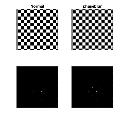
Fig. 55 Checkerboard pattern and simulated far-field (left) and the same checkerboard pattern after using the phaseblur() function (right).

otslm.tools.phaseblur(pattern, varargin)

Simulate pixel phase blurring

Usage

pattern = phaseblur(pattern, …) applies Gaussian blur to the pattern.

Parameters

• pattern (numeric) – pattern to blur

Optional named arguments

• colormap – colormap to apply before/after blurring. For a list of valid values, see colormap(). (default: [])
• invmap (logical) – apply inverse colormap at end (default: true)
• sigma (numeric) – size of the Gaussian kernel

volume2hologram

otslm.tools.volume2hologram(volume, varargin)

Generate hologram from 3-D volume by un-mapping the Ewald sphere

This function is only the inverse of hologram2volume() when interpolation use_weight is disabled and there is no blurring.

Usage

hologram = volume2hologram(volume, …) calculates the overlap of the Ewald sphere with the volume and projects it to a 2-D hologram.

Parameters

• volume (numeric) – 3-D volume to un-map

Optional named arguments

• ‘interpolate’ (logical) – interpolate between the nearest two pixels in the z-direction. (default: True)
• ‘padding’ (numeric) – padding in the axial direction (default 0).
• ‘focal_length’ (numeric) – focal length in pixels (default: estimated from z)
• ‘use_weight’ (logical) – use weights when sampling interpolated pixels

See also hologram2volume() and prop.FftEwaldForward.

castValue

This function is used to convert from logical patterns to another data type, such as double or integer. It is mainly used by functions which create binary masks including simple.aperture() and simple.step(). When the resulting pattern is used for indexing another pattern, the output should be logical. However, if the resulting pattern corresponds to phase or amplitude values, this function can be used to perform the cast.

For example, to convert from a logical pattern to a pattern with two discrete integer levels, we could do

in = [false(3, 3), true(3, 3)];
out = otslm.tools.castValue(in, uint8([0, 27]));

% Check that the output class matches the desired class (uint8)
disp(class(out));

otslm.tools.castValue(pattern, value)

Convert from logical pattern to specified value range

Usage

pattern = castValue(pattern, value)

Parameters

• pattern (logical) – the pattern to be converted
• value (numeric) – values for logical false and logical true pattern values. Should be either a 2 element vector [false_value, true_value].or an empty array to leave the values as logical.

lensesAndPrisms

This function implements the lenses and prisms algorithm. The algorithm can be used to generate multiple spots by adding the complex amplitude of each pattern together. The location of each spot is controlled using a lens (for axial position) or a linear grating (prism, for radial positioning). The algorithm can be implemented in just a few lines of code using the toolbox:

sz = [128, 128];

lin1 = otslm.simple.linear(sz, [10, 5]);
len1 = otslm.simple.spherical(sz, sz(1)*2);

lin2 = otslm.simple.linear(sz, [-5, 15]);
len2 = otslm.simple.spherical(sz, -sz(1)*2.7);

pattern = otslm.tools.combine({lin1+len1, lin2+len2}, 'method', 'super');

However, this requires each pattern to be stored in memory until they can be combined in a single call to combine(). This can become a problem when hundreds of patterns need to be combined or if running on hardware with limited memory such as a GPU.

The lensesAndPrisms() function is a more memory efficient implementation of the above. Firstly, it performs the combination after each pattern has been created, removing the need to store all the component patterns. Further, instead of calculating multiple linear gratings and spherical lenses, the function calculates a single x, y and lens pattern and scales these patterns to generate a component pattern. In code, the operation performed is

% Locations of 2 spots (3x2 matrix)
xyz = [1, 2, 3; 4, 5, 6].';

for ii = 1:size(xyz, 2)
   pattern = pattern + exp(1i*2*pi* ...
      (xyz(3, ii)*lens + xyz(1, ii)*xgrad + xyz(2, ii)*ygrad));
end

To use the function, we simply need to pass in a matrix for the spot locations. Additionally, we could pass in weights for the different components or custom patterns for the lens and gratings. Example output is shown in Fig. 56.

sz = [100, 100];
xyz = [10, 5, 0.1; -3, -2, -0.2] ./ sz(1);
pattern = otslm.tools.lensesAndPrisms(sz, xyz.');

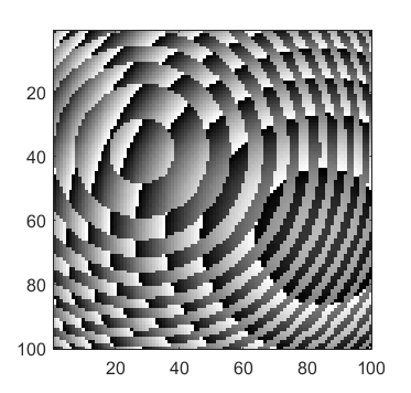
Fig. 56 Example output from lensesAndPrisms().

otslm.tools.lensesAndPrisms(sz, xyz, varargin)

Generates a hologram using the Lenses and Prisms algorithm

This function has the same affect as using multiple linear gratings and spherical lenses combined using otslm.tools.combine. The advantage of this function is a smaller memory footprint.

Usage

pattern = lensesAndPrisms(sz, xyz, …) The output pattern is in the range [0, 1). If supplied, the lens, xgrad and ygrad functions should have range [0, 1).

Parameters

• sz (size) – size of the pattern [rows, cols]
• xyz (numeric) – 3xN matrix for target spot locations. Each column describes a different target, the first two rows describe the linear gradient and the final row describes the lens magnitude.

Optional named parameters

• ‘lens’ – pattern to use for lens. (default: xx^2 + yy^2 where xx and yy are from otslm.simple.grid)
• ‘xgrad’ – pattern to use for x gradient. (default: xx from otslm.simple.grid)
• ‘ygrad’ – pattern to use for y gradient. (default: yy from otslm.simple.grid)
• ‘amplitude’ – vector of amplitudes for each location
• ‘gpuArray’ (logical) – True if the result should be a gpuArray

make_beam

This function combines the amplitude and phase image into a single complex amplitude pattern. Mathematically, the function does

\[U = I \times A \times \exp(i\phi)\]

where \(I\) is the incident illumination, \(\phi\) is the phase and \(A\) is the amplitude.

The function handles both 2-D patterns and 3-D volumes as well as a bunch of the size of the patterns and default values for any empty inputs.

otslm.tools.make_beam(phase, varargin)

Combine the phase, amplitude and incident patterns.

Usage

U = make_beam(phase, …) converts the phase pattern with a 2*pi range into a complex field amplitude. If phase is already complex the result is U = phase.

Parameters

• phase (numeric) – pattern to convert

Named parameters

• incident (numeric) – incident illumination.
• amplitude (numeric) – specify amplitude of the field. Only used when phase is a real matrix.