simple Package

This page contains a description of the functions contained in the otslm.simple package. These functions typically have analytic expressions and the functionality can be implemented in just a few lines of code. The implementation in the toolbox contains additional inputs to help with things like centring the patterns or generating the grids.

Most of these functions take as input the size of the image to generate, a two or three element vector with the width and height of the device; and parameters specific to the method. They produce one or more matlab matrices with the specified size. For example, a checkerboard image with 100 rows and 50 columns could be created with:

rows = 100;
cols = 50;
sz = [rows, cols];
im = otslm.simple.checkerboard(sz);
imagesc(im);
disp(size(im));

The functions have been grouped into categories: Lens functions, Beams, Gratings, 3-D functions and Miscellaneous. This is a very general and non-unique grouping. The output of many of these functions can be placed directly on a spatial light modulator as a phase or amplitude masks, or output of multiple functions can be combined using functions in the tools Package or Matlab operations on arrays (e.g., array addition or logical indexing).

Lens functions

These functions produce a single array. These arrays can be used to describe the phase functions of different lenses. Most of these functions support 1-D or 2-D variants, for instance, the spherical function can be used to create a cylindrical or spherical lens.

aspheric

otslm.simple.aspheric(sz, radius, kappa, varargin)

Generates a aspherical lens. The equation describing the lens is

\[z(r) = \frac{r^2}{ R ( 1 + \sqrt{1 - (1 + \kappa) r^2/R^2})} + \sum_{i=2}^N \alpha_i r^{2i} + \delta\]

where \(R\) is the radius of the lens, \(\kappa\) determines if the lens shape:

• <-1 – hyperbola
• -1 – parabola
• (-1, 0) – ellipse (surface is a prolate spheroid)
• 0 – sphere
• > 0 – ellipse (surface is an oblate spheroid)

and the \(\alpha\)’s corresponds to higher order corrections and \(\delta\) is a constant offset.

Usage

pattern = aspheric(sz, radius, kappa, …) generates a aspheric lens described by radius and conic constant centred in the image.

Parameters

• sz – size of the pattern [rows, cols]
• radius – Radius of the lens \(R\)
• kappa – conic constant \(\kappa\)

Optional named parameters

• ‘alpha’ [a1, …] – additional parabolic correction terms
• ‘delta’ offset – offset for the final pattern (default: 0.0)
• ‘scale’ scale – scaling value for the final pattern
• ‘background’ img – Specifies a background pattern to use for values outside the lens. Can be a matrix; a scalar, in which case all values are replaced by this value; or a string with ‘random’ or ‘checkerboard’ for these patterns.
• ‘centre’ [x, y] – centre location for lens (default: sz/2)
• ‘offset’ [x, y] – offset after applying transformations
• ‘type’ type – is the lens cylindrical or spherical (1d or 2d)
• ‘aspect’ aspect – aspect ratio of lens (default: 1.0)
• ‘angle’ angle – Rotation angle about axis (radians)
• ‘angle_deg’ angle – Rotation angle about axis (degrees)
• ‘gpuArray’ bool – If the result should be a gpuArray

axicon

otslm.simple.axicon(sz, gradient, varargin)

Generates a axicon lens. The equation describing the lens is

\[z(r) = -G |r|\]

where \(G\) is the gradient of the lens.

Usage

pattern = axicon(sz, gradient, …)

Parameters

• sz – size of the pattern [rows, cols]
• gradient – gradient of the lens \(G\)

Optional named parameters

• ‘centre’ [x, y] – centre location for lens (default: sz/2)
• ‘offset’ [x, y] – offset after applying transformations
• ‘type’ type – is the lens cylindrical or spherical (1d or 2d)
• ‘aspect’ aspect – aspect ratio of lens (default: 1.0)
• ‘angle’ angle – Rotation angle about axis (radians)
• ‘angle_deg’ angle – Rotation angle about axis (degrees)
• ‘gpuArray’ bool – If the result should be a gpuArray

Example (see also Fig. 36):

sz = [128, 128];
gradient = 0.1;
im = otslm.simple.axicon(sz, gradient);

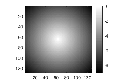
Fig. 36 Example of a axicon lens.

cubic

otslm.simple.cubic(sz, varargin)

Generates cubic phase pattern for Airy beams. The phase pattern is given by

\[f(x, y) = (x^3 + y^3)s^3\]

where \(s\) is a scaling factor.

Usage

pattern = cubic(sz, …) generates a cubic pattern according to

Parameters

• sz (size) – size of the pattern [rows, cols]

Optional named parameters

• scale (numeric) – Scaling factor for pattern.
• centre (numeric) – Centre location for lens (default: sz/2)
• offset (numeric) – Offset after applying transformations [x,y]
• type (enum) – Cylindrical 1d or spherical 2d
• aspect (numeric) – aspect ratio of lens (default: 1.0)
• angle (numeric) – Rotation angle about axis (radians)
• angle_deg (numeric) – Rotation angle about axis (degrees)
• gpuArray (logical) – If the result should be a gpuArray

Example (see also Fig. 37):

sz = [128, 128];
im = otslm.simple.cubic(sz);

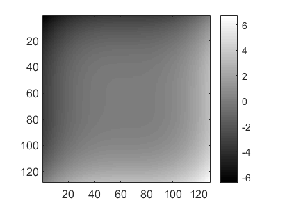
Fig. 37 Example of a cubic function.

spherical

otslm.simple.spherical(sz, radius, varargin)

Generates a spherical lens pattern. The equation describing the lens is

\[z(r) = \frac{R}{|R|} \frac{A}{r} \sqrt{R^2 - r^2}\]

where \(A\) is a scaling factor and \(R\) is the lens radius. Imaginary values are undefined and can be replaced by another value.

Usage

pattern = spherical(sz, radius, …) generates a spherical pattern with values from 0 (at the edge) and 1*sign(radius) (at the centre).

Parameters

• sz – size of the lens
• radius – radius of the lens \(R\)

Optional named arguments

• ‘delta’ offset – offset for pattern (default: -sign(radius))
• ‘scale’ scale – scaling value for the final pattern
• ‘background’ img – Specifies a background pattern to use for values outside the lens. Can also be a scalar, in which case all values are replaced by this value; or a string with ‘random’ or ‘checkerboard’ for these patterns.
• ‘centre’ [x, y] – centre location for lens
• ‘offset’ [x, y] – offset after applying transformations
• ‘type’ type – is the lens cylindrical or spherical (1d or 2d)
• ‘aspect’ aspect – aspect ratio of lens (default: 1.0)
• ‘angle’ angle – Rotation angle about axis (radians)
• ‘angle_deg’ angle – Rotation angle about axis (degrees)
• ‘gpuArray’ bool – If the result should be a gpuArray

See also aspheric().

The following example creates a spherical lens with radius 128 pixels, as shown in Fig. 38. The lens is centred in the pattern and a checkerboard pattern is used for values outside the lens.

sz = [256, 256];
radius = 128;
background = otslm.simple.checkerboard(sz);
im = otslm.simple.spherical(sz, radius, 'background', background);

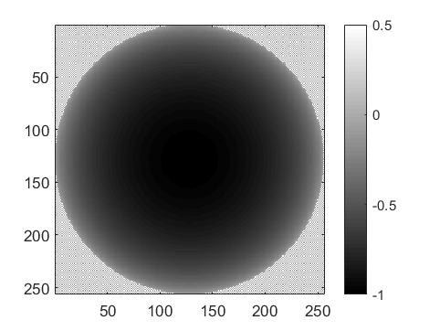
Fig. 38 Example of a spherical lens.

parabolic

otslm.simple.parabolic(sz, alphas, varargin)

Generates a parabolic lens pattern. The equation describing this lens is

\[z(r) = \alpha_1*r^2 + \alpha_2*r^4 + \alpha_3*r^6 + ...\]

where \(\alpha_n\) are the polynomial coefficients.

Usage

pattern = parabolic(sz, alphas, …) generates a parabolic lens.

Parameters

• sz (size) – size of pattern [rows, cols]
• alphas – array of polynomial coefficients \(\alpha_n\)

The default centre for the lens is the centre of the pattern, this can be modified with named parameters.

See also aspheric() for more information and named parameters.

gaussian

otslm.simple.gaussian(sz, sigma, varargin)

Generates a Gaussian pattern. A Gaussian pattern can be used as a lens or as the intensity profile for the incident illumination. The equation describing the pattern is

\[z(r) = A \exp{-r^2/(2\sigma^2)}\]

where \(A\) is a scaling factor and \(\sigma\) is the radius of the Gaussian.

Usage

pattern = gaussian(sz, sigma, …)

Parameters

• sz (numeric) – size of the pattern [rows, cols]
• sigma (numeric) – radius of the Gaussian \(\sigma\)

Optional named parameters

• ‘scale’ (numeric) – scaling value \(A\) (default: 1).
• ‘centre’ [x, y] – centre location for lens (default: sz/2)
• ‘offset’ [x, y] – offset after applying transformations
• ‘type’ type – is the lens cylindrical or spherical (1d or 2d)
• ‘aspect’ aspect – aspect ratio of lens (default: 1.0)
• ‘angle’ angle – Rotation angle about axis (radians)
• ‘angle_deg’ angle – Rotation angle about axis (degrees)
• ‘gpuArray’ bool – If the result should be a gpuArray

Example usage (see also Fig. 39):

sz = [128, 128];
sigma = 64;
im = otslm.simple.gaussian(sz, sigma, 'scale', 2.0);
imagesc(im);

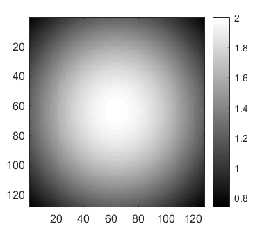
Fig. 39 Example output from gaussian().

Beams

These functions can be used to calculate the amplitude and phase patterns for different kinds of beams. To generate these kinds of beams, and other arbitrary beams, both the amplitude and phase of the beam needs to be controlled. This can be achieved by generating a phase or amplitude pattern which combines the phase and amplitude patterns produced by these functions, for details see the Advanced Beams example and otslm.tools.finalize().

bessel

otslm.simple.bessel(sz, mode, varargin)

Generates the phase and amplitude patterns for Bessel beams

Usage

pattern = bessel(sz, mode, …) generates the phase pattern for a particular order Bessel beam.

[phase, amplitude] = bessel(…) also calculates the signed amplitude of the pattern in addition to the phase.

Parameters

• sz – size of the pattern [rows, cols]
• mode (integer) – bessel function mode

Optional named parameters:

• ‘scale’ scale – radial scaling factor for pattern
• ‘centre’ [x, y] – centre location for lens (default: sz/2)
• ‘offset’ [x, y] – offset after applying transformations
• ‘type’ type – is the lens cylindrical or spherical (1d or 2d)
• ‘aspect’ aspect – aspect ratio of lens (default: 1.0)
• ‘angle’ angle – Rotation angle about axis (radians)
• ‘angle_deg’ angle – Rotation angle about axis (degrees)
• ‘gpuArray’ bool – If the result should be a gpuArray

hgmode

Hermite-Gaussian (HG) beams are solutions to the paraxial wave equation in Cartesian coordinates. Beams are described by two mode indices.

otslm.simple.hgmode(sz, xmode, ymode, varargin)

Generates the phase pattern for a HG beam

Usage

pattern = hgmode(sz, xmode, ymode, …) generates the phase pattern with x and y mode numbers.

[phase, amplitude] = hgmode(…) also calculates the signed amplitude of the pattern in addition to the phase.

Parameters

• sz – size of the pattern
• xmode – HG mode order in the x-direction
• ymode – HG mode order in the y-direction

Optional named parameters

• ‘scale’ scale – scaling factor for pattern
• ‘centre’ [x, y] – centre location for lens (default: sz/2)
• ‘offset’ [x, y] – offset after applying transformations
• ‘aspect’ aspect – aspect ratio of lens (default: 1.0)
• ‘angle’ angle – Rotation angle about axis (radians)
• ‘angle_deg’ angle – Rotation angle about axis (degrees)
• ‘gpuArray’ bool – If the result should be a gpuArray

lgmode

Laguerre-Gaussian (LG) beams are solutions to the paraxial wave equation in cylindrical coordinates.

otslm.simple.lgmode(sz, amode, rmode, varargin)

Generates the phase pattern for a LG beam

Usage

pattern = lgmode(sz, amode, rmode, …) generates phase pattern.

[phase, amplitude] = lgmode(…) also generates the amplitude pattern.

Parameters

• sz – size of the pattern
• amode – azimuthal order
• rmode – radial order

Optional named parameters

• ‘radius’ radius – scaling factor for radial mode rings
• ‘p0’ p0 – incident amplitude correction factor Should be 1.0 (default) for plane wave illumination (w_i = Inf), for Gaussian beams should be p0 = 1 - radius^2/w_i^2. See Lerner et al. (2012) for details.
• ‘centre’ [x, y] – centre location for lens (default: sz/2)
• ‘offset’ [x, y] – offset after applying transformations
• ‘aspect’ aspect – aspect ratio of lens (default: 1.0)
• ‘angle’ angle – Rotation angle about axis (radians)
• ‘angle_deg’ angle – Rotation angle about axis (degrees)
• ‘gpuArray’ bool – If the result should be a gpuArray

In order to generate pure LG beams it is necessary to control both the beam amplitude and phase. However, if the purity of the beam is not important then the phase pattern is often sufficient to generate the desired beam shape.

igmode

Ince-Gaussian (IG) beams are solutions to the paraxial wave equation in elliptical coordinates. The IG modes for a complete basis in elliptic coordinates. When the ellipticity parameter is infinite, IG beams are equivalent to HG beams, and when the ellipticity approaches 0, IG beams are equivalent to LG beams.

otslm.simple.igmode(sz, even, modep, modem, elipticity, varargin)

Generates phase and amplitude patterns for Ince-Gaussian beams

Ince-Gaussian beams are described in Bandres and Gutirrez-Vega (2004).

Warning

This function is a work-in-progress and may not produce clean output.

Usage

pattern = igmode(sz, even, modep, modem, elipticity, …)

[phase, amplitude] = igmode(…) also calculates the signed amplitude of the pattern in addition to the phase.

Parameters

• even – True for even parity
• modep – polynomial order p (integer: 0, 1, 2, …)
• modem – polynomial degree m (\(0 \leq m \leq p\))
• elipticity – elipticity of the coordinates.

Optional named parameters

• ‘scale’ scale – scaling factor for pattern
• ‘centre’ [x, y] – centre location for lens (default: sz/2)
• ‘offset’ [x, y] – offset after applying transformations
• ‘aspect’ aspect – aspect ratio of lens (default: 1.0)
• ‘angle’ angle – Rotation angle about axis (radians)
• ‘angle_deg’ angle – Rotation angle about axis (degrees)
• ‘gpuArray’ bool – If the result should be a gpuArray

This function uses code from Miguel Bandres, see source code for information about copyright/license/distribution.

Gratings

These functions can be used to create periodic patterns which can be used to create diffraction gratings.

linear

otslm.simple.linear(sz, spacing, varargin)

Generates a linear gradient. The pattern is described by

\[f(x) = \frac{1}{D} x\]

where the gradient is \(1/D\). For a periodic grating with maximum height of 1, \(D\) corresponds to the grating spacing.

Usage

pattern = linear(sz, spacing, …)

Parameters

• sz (numeric) – size of pattern [rows, cols]
• spacing – inverse gradient \(D\)

Optional named parameters

• ‘centre’ [x, y] – centre location for lens (default: [1, 1])
• ‘offset’ [x, y] – offset after applying transformations
• ‘aspect’ aspect – aspect ratio of lens (default: 1.0)
• ‘angle’ angle – Rotation angle about axis (radians)
• ‘angle_deg’ angle – Rotation angle about axis (degrees)
• ‘gpuArray’ bool – If the result should be a gpuArray

To generate a linear grating (a saw-tooth grating) you need to take the modulo of this pattern. This is done by otslm.tools.finalize() but can also be done explicitly with:

sz = [40, 40];
spacing = 10;
im = mod(otslm.simple.linear(sz, spacing, 'angle_deg', 45), 1);

Fig. 40 shows example output.

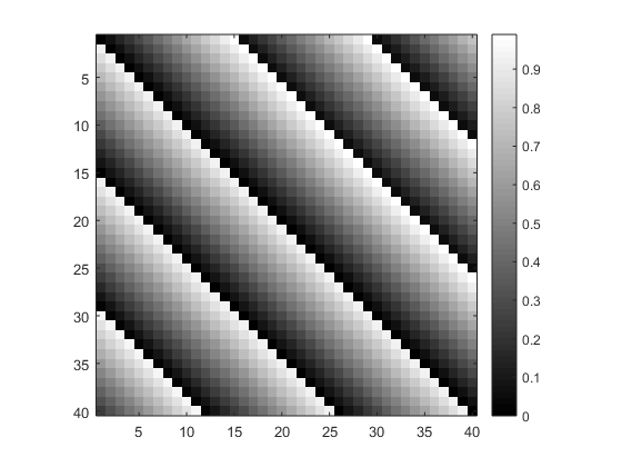
Fig. 40 Example output from linear().

Spacing can be a single number or two numbers for the spacing in the x and y directions. For an example of how linear() can be used to shift the beam focus, see Gratings and Lens LiveScript.

sinusoid

otslm.simple.sinusoid(sz, period, varargin)

Generates a sinusoidal grating. The function for the pattern is

\[f(x) = A\sin(2\pi x/P) + \delta\]

Where \(A\) is the scale, \(\delta\) is the mean, and \(P\) is the period.

This function can create a one dimensional grating in polar (circular) coordinates, in linear coordinates, or a mixture of two orthogonal gratings, see the types parameters for information.

Usage

pattern = sinusoid(sz, period, …) generates a sinusoidal grating with the default scale of 0.5 and default mean of 0.5.

Parameters

• sz (numeric) – size of pattern [rows, cols]
• period (numeric) – period \(P\)

Optional named parameters

• ‘scale’ (numeric) – pattern scale \(A\) (default: 1)
• ‘mean’ (numeric) – offset for pattern \(\delta\) (default: 0.5)
• ‘type’ (enum) – the type of sinusoid pattern to generate

• ‘1d’ – one dimensional (default)
• ‘2d’ – circular coordinates
• ‘2dcart’ – multiple of two sinusoid functions at 90 degree angle supports two period values [ Px, Py ].

• ‘centre’ [x, y] – centre location for lens
• ‘offset’ [x, y] – offset after applying transformations
• ‘aspect’ aspect – aspect ratio of lens (default: 1.0)
• ‘angle’ angle – Rotation angle about axis (radians)
• ‘angle_deg’ angle – Rotation angle about axis (degrees)
• ‘gpuArray’ bool – If the result should be a gpuArray

Fig. 41 shows different types of sinusoid gratings supported by the function.

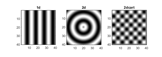
Fig. 41 Example of different sinusoid gratings generated using sinusoid().

Example usage (see also Fig. 42):

sz = [40, 40];
period = 10;
im = sinusoid(sz, period);

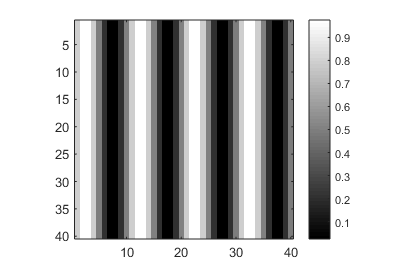
Fig. 42 Example output from sinusoid().

Miscellaneous

Various functions for generating patterns not described in other sections. This includes the grid() and aperture() functions which are used to create the grids and masks used by other toolbox functions.

aperture

otslm.simple.aperture(sz, dimension, varargin)

Generates different shaped aperture patterns/masks

Usage

pattern = aperture(sz, dimension, …) creates a circular aperture with radius given by parameter dimension. Array is logical array.

Parameters

• sz – size of the pattern [rows, cols]
• dimension – List of numbers describing the aperture size. Lens of the list depends on the aperture shape. For a circle dimensions is one element, the radius of the circle.

Optional named parameters

• ‘shape’ – Shape of aperture to generate. See supported shapes bellow.
• ‘value’ [l, h] – values for off and on regions (default: [])
• ‘centre’ [x, y] – centre location for pattern
• ‘offset’ [x, y] – offset in rotated coordinate system
• ‘aspect’ (num) – aspect ratio of lens (default: 1.0)
• ‘angle’ (num) – Rotation angle about axis (radians)
• ‘angle_deg’ (num) – Rotation angle about axis (degrees)
• ‘gpuArray’ (logical) – If the result should be a gpuArray

Supported shapes [dimensions]

• ‘circle’ [radius] – Pinhole/circular aperture
• ‘square’ [width] – Square with equal sides
• ‘rect’ [w, h] – Rectangle with width and height
• ‘ring’ [r1, r2] – Ring specified by inner and outer radius

Fig. 43 shows examples of different apertures.

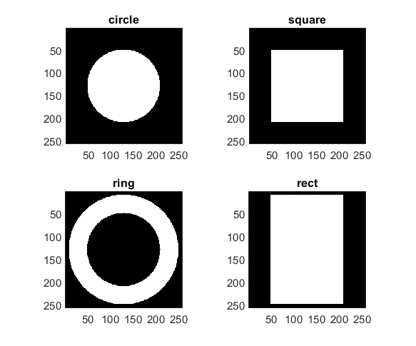
Fig. 43 Example of different aperture types generated by aperture().

Logical arrays can be used to mask parts of other arrays. This can be useful for creating composite images, for example (see also Fig. 44):

sz = [256, 256];
im = otslm.simple.linear(sz, 256);
chk = otslm.simple.checkerboard(sz);
app = otslm.simple.aperture(sz, 80);
im(app) = chk(app);

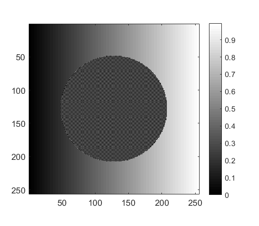
Fig. 44 Example of using aperture() to generate logical arrays for masking two patterns.

aberrationRiMismatch

otslm.simple.aberrationRiMismatch(sz, n1, n2, alpha, varargin)

Calculates aberration for a plane interface refractive index mismatch.

The aberration can be described using geometric optics, see Booth et al., Journal of Microscopy, Vol. 192, Pt 2, Nov. 1998. This function calculates the pattern according to

\[z(r) = d f(r) n_1 \sin\alpha\]

where

\[f(r) = \sqrt{\csc^2\beta - r^2} - \sqrt{\csc^2\alpha - r^2},\]

\(d\) is the depth into medium 2, \(n_1, n_2\) are the refractive indices in the mediums, \(n_1\sin\alpha = n_2 \sin\beta\) and \(\alpha\) is the maximum capture angle of the lens which is related to the numerical aperture by \(n_1 \sin\alpha\).

The focus is located in medium 2, which is separated from medium 1 and the lens by a plane interface.

Usage

pattern = aberrationRiMismatch(sz, n1, n2, alpha, …)

Parameters

• sz (size) – size of pattern [rows, cols]
• n1 (numeric) – refractive index of medium 1
• n2 (numeric) – refractive index of medium 2
• alpha (numeric) – maximum capture angle of lens (radians)

Optional named parameters

• radius (numeric) – radius of aperture. Default min(sz)/2.
• depth (numeric) – depth of focus into medium 2 (units of wavelength in medium). Default 1.0.
• background (numeric|enum) – Specifies a background pattern to use for values outside the lens. Can also be a scalar, in which case all values are replaced by this value; or a string with ‘random’ or ‘checkerboard’ for these patterns.
• ‘centre’ [x, y] – centre location for lens
• ‘offset’ [x, y] – offset after applying transformations
• ‘aspect’ aspect – aspect ratio of lens (default: 1.0)
• ‘angle’ angle – Rotation angle about axis (radians)
• ‘angle_deg’ angle – Rotation angle about axis (degrees)
• ‘gpuArray’ bool – If the result should be a gpuArray

See also examples.liveScripts.booth1998.

Example usage (see also Fig. 45):

sz = [512, 512];
n1 = 1.5;
n2 = 1.33;
NA = 0.4;
alpha = asin(NA/n1);
pattern = otslm.simple.aberrationRiMismatch(sz, ...
    n1, n2, alpha, 'depth', 2.0);

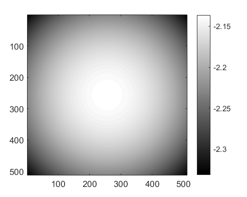
Fig. 45 Example output from aberrationRiMismatch().

zernike

zernike() generates a pattern based on the Zernike polynomials. The Zernike polynomials are a complete basis of orthogonal functions across a circular aperture. This makes them useful for describing beams or phase corrections to beams at the back-aperture of a microscope objective.

otslm.simple.zernike(sz, m, n, varargin)

Generates a pattern based on the zernike polynomials.

The polynomials are parameterised by two integers, \(m\) and \(n\). \(n\) is a positive integer, and \(|m| \leq n\).

Usage

pattern = zernike(sz, m, n, …)

Parameters

• sz (numeric) – size of the pattern [rows, cols]
• m (numeric) – polynomial order parameter (integer)
• n (numeric) – polynomial order parameter (integer)

Optional named parameters

• ‘scale’ scale – scaling value for the final pattern
• ‘rscale’ rscale – radius scaling factor (default: min(sz)/2)
• ‘outside’ val – Value to use for outside points (default: 0)
• ‘centre’ [x, y] – centre location for lens (default: sz/2)
• ‘offset’ [x, y] – offset after applying transformations
• ‘aspect’ aspect – aspect ratio of lens (default: 1.0)
• ‘angle’ angle – Rotation angle about axis (radians)
• ‘angle_deg’ angle – Rotation angle about axis (degrees)
• ‘gpuArray’ bool – If the result should be a gpuArray

See also examples.liveScripts.booth1998.

Example usage (see also Fig. 46):

n = 4;
m = 2;
sz = [512, 512];
im = otslm.simple.zernike(sz, m, n);

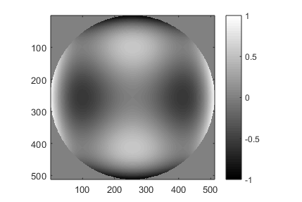
Fig. 46 Example output from zernike().

hadamard

Hadamard matrices can be used as a discrete binary orthogonal basis in Cartesian coordinates for applications such as single pixel imaging. This function generates images representing rows of a Hadamard matrix. These patterns can be used as an alternative to Fourier single-pixel imaging, for example and comparison see

Zibang Zhang et al., Hadamard single-pixel imaging versus Fourier single-pixel imaging. Vol. 25, Issue 16, pp. 19619-19639 (2017) https://doi.org/10.1364/OE.25.019619

otslm.simple.hadamard(sz, u, v, varargin)

Generate a two dimensional pattern based on a row of the Hadamard matrix.

These patterns form an orthogonal basis of discrete binary patterns in Cartessian coordinates. They can be used for implementing various imaging schemes such as Hadamard Single Pixel imaging.

Usage

pattern = otslm.simple.hadamard(sz, u, v, …) constructs a single square Hadamard basis pattern starting at row 1 column 1.

Parameters

• sz (2x1 numeric) – size of the output pattern. The Hadamard patterns should be square with width N satisfying the condition either N, N/12 or N/20 is a power of 2; otherwise, the total number of pixels should be a number satisfying the same condition. By default, the patterns are assumed to be square and N = 2^floor(log2(min(sz))). When sz is larger than NxN, extra values are padded with padding_value.
• u, v (numeric scalar) – row and column index for Hadamard pattern. For square patterns, these should be in the range [1, N], for linear indexed patterns, v can be set to 1 and u is the pixel index. Alternatively, for linear indexed patterns, u, v should be able to be passed to sub2ind with size equal to target_size.

Optional named arguments

• padding_value (numeric) – Value to use for padding for values outside the target_size region. Default: 0.

• target_size (2x1 numeric) – Target size for the 2-D Hadamard pattern. See sz parameter for details. Target size can be non-square, in which case linear indexing is used. Default: [1,1] .* 2^floor(log2(min(sz))).

• value [l, h] – Lower and upper values for pattern. Default: [0, 1].

• indexing (enum) – Type of indexing to use. Either ‘square’ or ‘linear’. Default: ‘square’ unless target_size is non-square.

• order (enum) – Ordering of patterns. - hadamard – Order the same as Matlab’s hadamard function. - bitrevorder – Applies bit reversal to u and v. - largetosmall – Orders patterns by the size of the solid region,

  large regions have lower u/v index, small regions have higher index. Should produce the same result at linear indexing with ‘hadamard’ ordering.

  Default: ‘largetosmall’ for square indexing, ‘hadamard’ for linear.

• centre [x, y] – centre location for pattern. Default: [] for top corner, i.e. target_size/2 + [0.5, 0.5].

• offset [x, y] – offset after applying transformations. Default: [0, 0].

• scale (numeric) – Scaling factor for the pattern. Either a scalar or 2 element vector for [x, y] scaling. Default: 1.0

• angle (numeric) – Rotation angle about axis (radians) (default: 0.0).

• angle_deg (numeric) – Rotation angle about axis (degrees).

• aspect (numeric) – Aspect ratio of pattern (default: 1.0)

Example usage (see also Fig. 47):

u = 2;
v = 3;
sz = [8, 20];
im = otslm.simple.hadamard(sz, u, v);

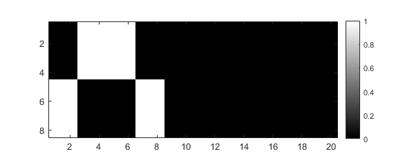
Fig. 47 Example output from hadamard(). The pattern corresponds to one row from a 16x16 Hadamard Matrix (i.e. product of two 8x8 Hadamard row vectors). Values outside the pattern have been filled with zeros.

sinc

otslm.simple.sinc(sz, radius, varargin)

Generates a sinc pattern. This pattern can be used to create a line shaped trap or as a model for the diffraction pattern from a aperture. The equation describing the pattern is

\[f(x) = \sin(\pi x/R)/(\pi x/R)\]

and 1 when x is zero; where \(R\) is the radius (scaling factor).

Usage

pattern = sinc(sz, radius, …)

Parameters

• sz (numeric) – size of the pattern [rows, cols]
• radius (numeric) – radial scaling factor

Optional named parameters

• ‘type’ type – the type of sinc pattern to generate

• ‘1d’ – one dimensional
• ‘2d’ – circular coordinates
• ‘2dcart’ – multiple of two sinc functions at 90 degree angle supports two radius values: radius = [ Rx, Ry ].

• ‘centre’ [x, y] – centre location for lens
• ‘offset’ [x, y] – offset after applying transformations
• ‘aspect’ aspect – aspect ratio of lens (default: 1.0)
• ‘angle’ angle – Rotation angle about axis (radians)
• ‘angle_deg’ angle – Rotation angle about axis (degrees)
• ‘gpuArray’ bool – If the result should be a gpuArray

Example usage (see also Fig. 48):

radius = 10;
sz = [100, 100];
im = otslm.simple.sinc(sz, radius);

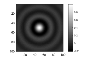
Fig. 48 Example output from sinc().

checkerboard

otslm.simple.checkerboard(sz, varargin)

Generates a checkerboard pattern. A checkerboard pattern with equal sized squares can be written mathematically as

\[f(x, y) = \mod(x + y, 2)\]

Usage

pattern = checkerboard(sz, …) creates a checkerboard with spacing of 1 pixel and values of 0 and 0.5.

Parameters

• sz – size of the pattern [rows, cols]

Optional named parameters

• ‘spacing’ spacing – Width of checks (default 1 pixel)
• ‘value’ [l,h] – Lower and upper values of checks (default: [0, 0.5])
• ‘centre’ [x, y] – centre location for lens (default: sz/2)
• ‘offset’ [x, y] – offset after applying transformations
• ‘type’ type – is the lens cylindrical or spherical (1d or 2d)
• ‘aspect’ aspect – aspect ratio of lens (default: 1.0)
• ‘angle’ angle – Rotation angle about axis (radians)
• ‘angle_deg’ angle – Rotation angle about axis (degrees)
• ‘gpuArray’ bool – If the result should be a gpuArray

Example usage (see also Fig. 49):

sz = [5,5];
im = otslm.simple.checkerboard(sz);
imagesc(im);

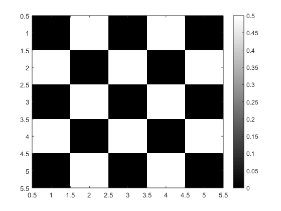
Fig. 49 Example output from checkerboard().

stripes

otslm.simple.stripes(sz, spacing, varargin)

Generates a stripe pattern

Generates a pattern with alternating evently spaced stripes with values of 0 and 0.5 (or a user defined value).

Usage

pattern = stripe(sz, spacing, …)

Parameters

• sz (numeric) – size of pattern [rows, cols]
• spacing (numeric) – width of stripes (scalar)

Optional named parameters

• ‘value’ [l,h] – Lower and upper values default: [0, 0.5]
• ‘centre’ [x, y] – centre location for lens default: [1, 1]
• ‘offset’ [x, y] – offset after applying transformations
• ‘aspect’ aspect – aspect ratio of lens (default: 1.0)
• ‘angle’ angle – Rotation angle about axis (radians)
• ‘angle_deg’ angle – Rotation angle about axis (degrees)
• ‘gpuArray’ bool – If the result should be a gpuArray

Example usage (see also Fig. 50):

sz = [10, 10];
im = otslm.simple.stripes(sz, 2);
imagesc(im);

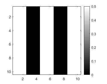
Fig. 50 Example output from stripes().

grid

otslm.simple.grid(sz, varargin)

Generates a grid of points similar to meshgrid.

This function is used by most other otslm.simple functions to create grids of Cartesian or polar coordinates. Without any optional parameters, this function produces a similar result to the Matlab meshgrid() function but with 0 centred at the centre of the image.

Usage

xx, yy = grid(sz, …)

xx, yy, rr, phi = grid(sz, …) calculates polar coordinates.

Parameters

• sz – size of the pattern [rows, cols]

Optional named parameters

• ‘centre’ [x, y] – centre location for lens (default: sz/2)
• ‘offset’ [x, y] – offset after applying transformations
• ‘type’ type – is the lens cylindrical or spherical (1d or 2d)
• ‘aspect’ aspect – aspect ratio of lens (default: 1.0)
• ‘angle’ angle – Rotation angle about axis (radians)
• ‘angle_deg’ angle – Rotation angle about axis (degrees)
• ‘gpuArray’ bool – If the result should be a gpuArray

Example usage (see also Fig. 51):

sz = [10, 10];
[xx, yy, rr, phi] = otslm.simple.grid(sz);

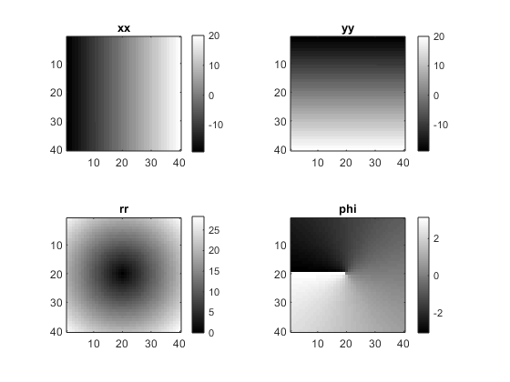
Fig. 51 Example output from grid().

random

otslm.simple.random(sz, varargin)

Generates a image filled with random noise. The function supports three types of noise: uniform, normally distributed, and binary.

Usage

pattern = random(sz, …) creates a pattern with uniform random noise values between 0 and 1. See the ‘type’ argument for other noise types.

Parameters

• sz – size of the pattern

Optional named parameters

• ‘range’ (numeric) – Range of values (default: [0, 1]).
• ‘type’ (enum) – Type of noise. Can be ‘uniform’, ‘gaussian’, or ‘binary’. (default: ‘uniform’)
• ‘gpuArray’ (logical) – If the result should be a gpuArray

Example (see also Fig. 52):

sz = [20, 20];
im = otslm.simple.random(sz, 'type', 'binary');

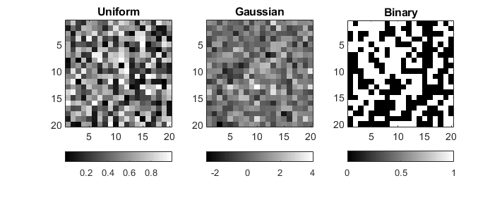
Fig. 52 Example output from random().

step

otslm.simple.step(sz, varargin)

Generates a step. The function is described by

\[ \begin{align}\begin{aligned}f(x) = 0 \qquad x < 0\\f(x) = 1 \qquad x \geq 0\end{aligned}\end{align} \]

Usage

pattern = step(sz, …) generates a step at the centre of the image.

Parameters

sz – size of the pattern

Optional named parameters

• ‘value’ [ l, h ] – low and high values of step (default: [0, 0.5])
• ‘centre’ [x, y] – centre location for pattern
• ‘offset’ [x, y] – offset in rotated coordinate system
• ‘aspect’ aspect – aspect ratio of lens (default: 1.0)
• ‘angle’ angle – Rotation angle about axis (radians)
• ‘angle_deg’ angle – Rotation angle about axis (degrees)
• ‘gpuArray’ bool – If the result should be a gpuArray

Example usage (see also Fig. 53):

sz = [5, 5];
im = otslm.simple.step(sz);

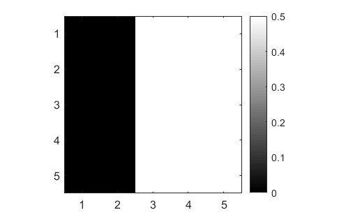
Fig. 53 Example output from step().

3-D functions

These functions generate a 3-D volume instead of a 2-D image. The size parameter is a 3 element vector for the x, y, z dimension sizes.

aperture3d

otslm.simple.aperture3d(sz, dimension, varargin)

Generate a 3-D volume similar to aperture(). Can be used to create a target 3-D volume for beam shape optimisation.

Usage

pattern = aperture3d(sz, dimension, …)

Properties

• sz – Size of the pattern [rows, cols, depth]
• dimensions – aperture dimensions (depends on aperture shape)

Optional named parameters

• ‘shape’ – Shape of aperture to generate. See supported shapes.
• ‘value’ [l, h] – values for off and on regions (default: [])
• ‘centre’ [x, y, z] – centre location for pattern
• ‘gpuArray’ (logical) – If the result should be a gpuArray

Supported shapes [dimensions]

• ‘sphere’ [radius] – Pinhole/circular aperture
• ‘cube’ [width] – Square with equal sides
• ‘rect’ [w, h, d] – Rectangle with width and height
• ‘shell’ [r1, r2] – Ring specified by inner and outer radius

grid3d

otslm.simple.grid3d(sz, varargin)

Generates a 3-D grid similar to grid()

Usage

[xx, yy, zz] = grid3d(sz, …) Equivalent to mesh grid.

[xx, yy, zz, rr, theta, phi] = grid3d(sz, …) Additionally, calculates spherical coordinates:

• rr – Distance from centre of pattern
• theta – polar angle, measured from +z axis [0, pi]
• phi – azimuthal angle, measured from +x towards +y axes [0, 2*pi)

Parameters

• sz – size of the pattern [rows, cols]

Optional named parameters

• ‘centre’ [x, y, z] – centre location for lens
• ‘gpuArray’ bool – If the result should be a gpuArray

gaussian3d

otslm.simple.gaussian3d(sz, sigma, varargin)

Generates a gaussian volume similar to gaussian().

The equation describing the lens is

\[z(r) = s \exp{-r^2/(2\sigma^2)}\]

where \(s\) is a scaling factor and \(\sigma\) describes the radius of the Gaussian distribution.

Usage

pattern = gaussian3d(sz, sigma, …)

Parameters

• sz – size of the pattern [rows, cols, depth]
• sigma – radius of the distribution \(\sigma\). Can be a 1 or 3 element vector for the radial or [x, y, z] scaling.

Optional named parameters

‘scale’ scale scaling value for the final pattern ‘centre’ [x, y] centre location for lens ‘gpuArray’ bool If the result should be a gpuArray

linear3d

otslm.simple.linear3d(sz, spacing, varargin)

Generates a linear gradient similar to linear()

Usage

pattern = linear3d(sz, spacing, …)

Parameters

• sz – size of pattern to generate
• spacing – Inverse slope (1/spacing). Can be a scalar or a 3 element vector.

Optional named parameters

• ‘centre’ [x, y, z] – centre location for pattern
• ‘gpuArray’ bool – If the result should be a gpuArray