Simple Beams
This page describes the examples.simple_beams example. This example
demonstrates some of the simpler hologram generation functions in the
toolbox.
Contents
Initial setup
The example starts by adding the OTSLM toolbox to the path. The
example script is in the otslm-directory/examples/ directory,
allowing us to specify the otslm-directory relative to the current
directory with ../
addpath('../');
We define a couple of properties for the patterns, starting with the
size of the patterns [512, 512] and the incident illumination we
will use for the simulation.
sz = [512, 512];

% incident = [];        % Incident beam (use default in visualize)
incident = otslm.simple.gaussian(sz, 150);  % Incident beam (gaussian)
% incident = ones(sz);  % Incident beam (use uniform illumination)
We use otslm.simple.gaussian() to create a Gaussian profile
for the incident illumination.
Alternatively we could just us the Matlab ones() function to
create a uniform incident illumination or load a gray-scale image from
a file.
The last part of the setup section defines a couple of functions for visualising the SLM patterns in the far-field.
o = 50;              % Region of interest size in output
padding = 500;        % Padding for FFT
zoom = @(im) im(round(size(im, 1)/2)+(-o:o), round(size(im, 2)/2)+(-o:o));
visualize = @(pattern) zoom(abs(otslm.tools.visualise(pattern, ...
    'method', 'fft', 'padding', padding, 'incident', incident)).^2);
This defines a function visualize which takes a pattern as input,
uses the otslm.tools.visualise() method to simulate what the
far-field looks like using the fast Fourier transform method, calculates the
absolute value squared (converts from the complex output of
otslm.tools.visualise() to an intensity image which we can plot with
imagesc()) and zooms into a region of interest in the far-field image.
This piece of code isn’t really part of the example, it is only included
to make the following sections more succinct. You could replace the use
of the visualize function in the sections below with a single call
the otslm.tools.visualise() and manually zoom into the resulting
image.
Exploring different simple beams
The remainder of the example explores different beams. This section describes each beam phase pattern and shows the expected output.
Zero phase pattern
When a constant (or zero) phase pattern is placed on the SLM, the resulting beam is unmodified (except for a constant phase factor which doesn’t affect the resulting intensity). When we visualise this beam, we should see the Fourier transform of the incident beam. If our incident beam is a Gaussian, we should see a Gaussian-like spot in the far-field, as shown in Fig. 3.
pattern = zeros(sz);
pattern = otslm.tools.finalize(pattern);
subplot(1, 2, 1), imagesc(pattern);
subplot(1, 2, 2), imagesc(visualize(pattern));
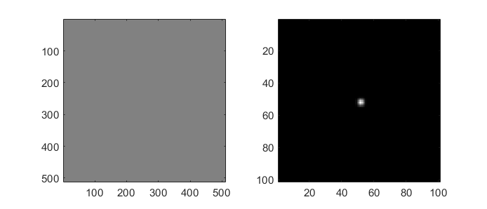
Fig. 3 A phase pattern with zero phase shift (left) and the resulting unchanged far-field intensity (right).
This example includes a call to otslm.tools.finalize(), for the zero
phase pattern this call is redundant. If you changed the pattern to a
constant uniform phase shift, for example 10.5*ones(sz),
otslm.tools.finalize() would apply mod(pattern, 1)*2*pi to the
pattern to ensure the pattern is between 0 and 2pi.
Linear grating
The linear grating can be used for shifting the focus of a beam in the
far-field. The linear grating acts like a tilted mirror, on the side of
the mirror where the path length is reduced the relative phase is less
than zero, on the side of the mirror where the path length is increased
the phase difference is larger. To create a linear grating you can use
the otslm.simple.linear() function. This function has two required
arguments, the pattern size and the grating spacing. The grating spacing
is proportional to the distance the beam is displaced in the far-field
and inversely proportional to the gradient of the pattern.
Fig. 4 shows a typical output.
pattern = otslm.simple.linear(sz, 40, 'angle_deg', 45);
pattern = otslm.tools.finalize(pattern);
subplot(1, 2, 1), imagesc(pattern);
subplot(1, 2, 2), imagesc(visualize(pattern));
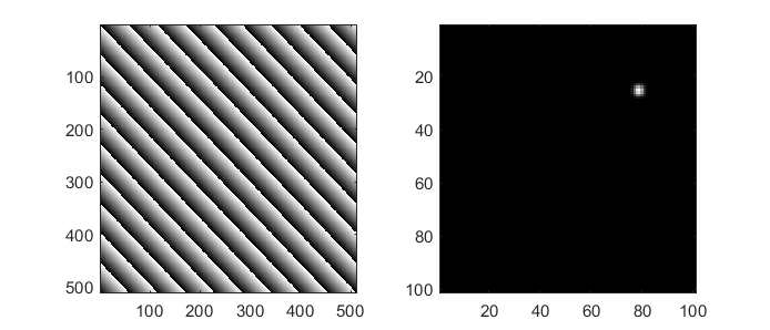
Fig. 4 A blazed grating generated using otslm.simple.linear()
and and the resulting far-field intensity pattern.
The otslm.simple.linear() function outputs a non-modulated pattern,
as shown in Fig. 5.
This makes it easier to combine the pattern with other
patterns without introducing artefacts from applying
mod(pattern, 1). Passing the pattern to otslm.tools.finalize()
applies the modulo to the pattern producing the recognisable blazed
grating pattern.
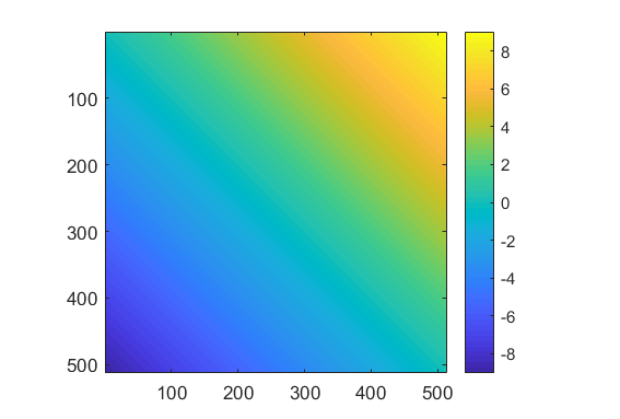
Fig. 5 Un-modulated output from otslm.simple.linear().
Spherical grating
To shift the beam focus along the axial direction we can use a lens
function. The toolbox includes a couple of simple
Lens functions, here we use
otslm.simple.spherical(). This function takes two required arguments:
the pattern size and lens radius. Values outside the lens radius are
invalid, we can choose how these values are represented using the
background optional argument, in this case we choose to replace
these values with a checkerboard pattern. The checkerboard pattern
diffracts light to high angles (outside the range of the cropping in the
visualize method).
By default, the spherical lens has a height of 1.
We can scale the height by multiplying the output by the desired scale,
this will scale the lens and the background pattern.
To avoid applying the scaling to the background pattern we can
use the scale optional argument.
Typical output is shown in Fig. 6.
pattern = otslm.simple.spherical(sz, 200, 'scale', 5, ...
    'background', 'checkerboard');
pattern = otslm.tools.finalize(pattern);
subplot(1, 2, 1), imagesc(pattern);
subplot(1, 2, 2), imagesc(visualize(pattern));
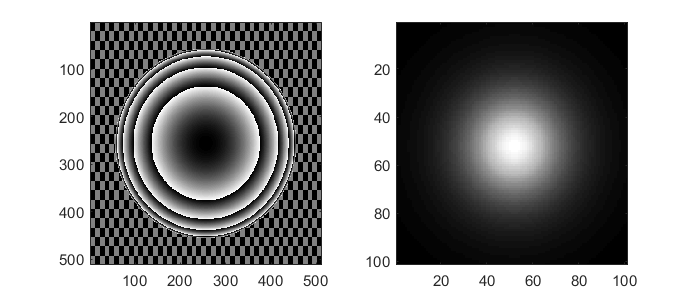
Fig. 6 Typical output and far-field intensity from the
otslm.simple.spherical() function.
The output has been modulated to produce the recognisable
Fresnel-style lens pattern.
The output of otslm.simple.spherical() is non-modulated, similar to
otslm.simple.linear() described above. Only when
otslm.tools.finalize`() is applied does the pattern look like a
Fresnel lens pattern.
LG Beam
The toolbox provides methods for generating the amplitude and phase
patterns for LG beams. To calculate the phase profile for an LG beam, we
can use otslm.simple.lgmode(). This function takes as inputs the
pattern size, azimuthal and radial modes and an optional scaling factor
for the radius of the pattern.
Typical output is shown in Fig. 7.
amode = 3;  % Azimuthal mode
rmode = 2;  % Radial mode
pattern = otslm.simple.lgmode(sz, amode, rmode, 'radius', 50);
pattern = otslm.tools.finalize(pattern);
subplot(1, 2, 1), imagesc(pattern);
subplot(1, 2, 2), imagesc(visualize(pattern));
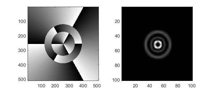
Fig. 7 Example output from otslm.simple.lgmode().
In order to generate a pure LG beam we need to be able to control both the amplitude and phase of the light. This can be achieved using separate devices for the amplitude and phase modulator or by mixing the amplitude pattern into the phase, as is described in the Advanced Beams example.
HG Beam
Amplitude and phase patterns can be calculated using the
otslm.simple.hgmode() function.
The output from this function is shown in Fig. 8.
This function takes as input the
pattern size and the two mode indices. There is also an optional
scale parameter for scaling the pattern. As with LG beams,
generation of pure HG beams requires control of both the phase and
amplitude of the light, see the Advanced Beams example for
more details.
pattern = otslm.simple.hgmode(sz, 3, 2, 'scale', 70);
pattern = otslm.tools.finalize(pattern);
subplot(1, 2, 1), imagesc(pattern);
subplot(1, 2, 2), imagesc(visualize(pattern));
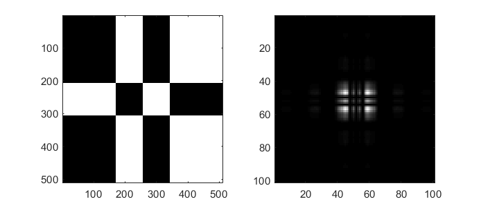
Fig. 8 Phase pattern (left) generated using the otslm.simple.hgmode()
method and the corresponding simulated far-field (right).
The simulated far-field doesn’t have any amplitude correction,
leading to a non-pure HG beam output.
Sinc pattern
A sinc amplitude pattern can be used to generate a line-shaped focal spot in the far-field. For phase-only SLMs, we need to encode the amplitude in the phase pattern, this can be achieved by mixing the pattern with a second phase pattern (as described in Advanced Beams), or for 1-D patterns we can encode the amplitude into the second dimension of the SLM (similar to Roichman and Grier, Opt. Lett. 31, 1675-1677 (2006)). In this example, we show the latter.
First we create the sinc profile using the otslm.simple.sinc()
function. This function takes two required arguments, pattern size and
the sinc radius. The function can generate both 1-dimensional and
2-dimensional sinc patterns, but for the 1-D encoding method we need a
1-dimensional pattern, as shown in Fig. 9.
radius = 50;
sinc = otslm.simple.sinc(sz, 50, 'type', '1d');
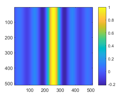
Fig. 9 1-dimensional sinc pattern output from otslm.simple.sinc().
To encode the 1-dimensional pattern into the second dimension of the SLM
we can use otslm.tools.encode1d(). This method takes a 2-D
amplitude image, the amplitude should be constant in one direction and
variable in the other direction. For the above image, the amplitude is
constant in the vertical direction and variable in the horizontal
direction. The method determines which pixels have a value greater than
the location of the pixel in the vertical direction. Pixels within this
range are assigned the phase of the pattern (0 for positive amplitude,
0.5 for negative amplitudes). Pixels outside this region should be
assigned another value, such as a checkerboard pattern. The encode
method also takes an optional argument to scale the pattern by, this can
be thought of as the ratio of pattern amplitude and device height.
[pattern, assigned] = otslm.tools.encode1d(sinc, 'scale', 200);

% Apply a checkerboard to unassigned regions
checker = otslm.simple.checkerboard(sz);
pattern(~assigned) = checker(~assigned);
We can then finalize and visualise our pattern to produce Fig. 10.
pattern = otslm.tools.finalize(pattern);
subplot(1, 2, 1), imagesc(pattern);
subplot(1, 2, 2), imagesc(visualize(pattern));
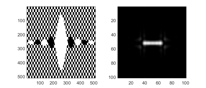
Fig. 10 Sinc pattern encoded with otslm.tools.encode1d().
Axicon lens
An axicon (cone shaped) lens can be useful for creating Bessel-like beams in the near-field. In the far-field, the light will have a ring-shaped profile, while in the near-field the light should have a Bessel-like profile. It is also possible to combine the axicon lens with an azimuthal gradient to generate Bessel-like beams with angular momentum. Example output is shown in Fig. 11.
radius = 50;
pattern = otslm.simple.axicon(sz, -1/radius);
pattern = otslm.tools.finalize(pattern);
subplot(1, 2, 1), imagesc(pattern);
subplot(1, 2, 2), imagesc(visualize(pattern));
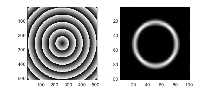
Fig. 11 Axicon pattern (left) and simulated far-field (right).
To see the Bessel-shaped profile, we need to look at the near-field. We
can use the otslm.tools.visualise()
method with a z offset to view
the near-field of the axicon, as shown in
Fig. 12.
im1 = otslm.tools.visualise(pattern, 'method', 'fft', 'trim_padding', true, 'z', 50000);
im2 = otslm.tools.visualise(pattern, 'method', 'fft', 'trim_padding', true, 'z', 70000);
im3 = otslm.tools.visualise(pattern, 'method', 'fft', 'trim_padding', true, 'z', 90000);
figure();
subplot(1, 3, 1), imagesc(zoom(abs(im1).^2)), axis image;
subplot(1, 3, 2), imagesc(zoom(abs(im2).^2)), axis image;
subplot(1, 3, 3), imagesc(zoom(abs(im3).^2)), axis image;
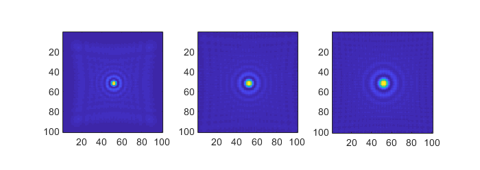
Fig. 12 Visualisation of the near-field of the axicon pattern
using otslm.tools.visualise() with three different
axial offsets.
Cubic lens
The cubic lens pattern otslm.simple.cubic()
can be used to create airy
beams.
Fig. 13 shows example output.
pattern = otslm.simple.cubic(sz);
pattern = otslm.tools.finalize(pattern);
subplot(1, 2, 1), imagesc(pattern);
subplot(1, 2, 2), imagesc(visualize(pattern));
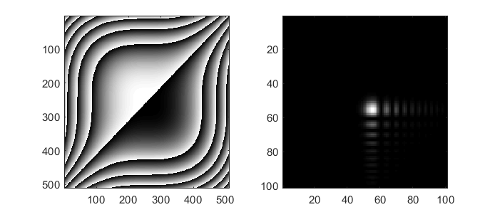
Fig. 13 Example output using otslm.simple.cubic().