Advanced Beams

This page describes the examples.advanced_beams example. This example demonstrates some of the more complex hologram generation capabilities in the toolbox including: combining multiple holograms, shaping the amplitude with a phase-only device, iterative algorithms, and binary amplitude patterns.

Note

Many of the images in this documentation include checkerboard patterns. The checkerboard pattern should have a width of 1 pixel to scatter light to high angles, however the lower resolution images shown in the documentation appear to have a courser checkerboard pattern as a result of a Moiré/aliasing effect. To use these patterns, we recommend generating higher resolution versions using the toolbox.

Initial setup

The start of the script defines parameters and functions for visualising the far-field of the SLM. This is mostly the same as the initial setup in the Beams example. Some of the advanced beams include a beam amplitude correction term to compensate for the non-uniform illumination of the pattern from the incident beam. The beam correction term is defined as

beamCorrection = 1.0 - incident + 0.5;
beamCorrection(beamCorrection > 1.0) = 1.0;

Amplitude control with a phase device

In the LG Beam and HG Beam examples in examples.simple_beams we noted how in order to create pure LG or HG beams we need to control both the phase and amplitude of the beam. In the Sinc pattern example we used the otslm.tools.encode1d() method to encode a 1-dimensional pattern into a 2-dimensional phase pattern. For encoding two dimensional phase patterns we need to create a mixture of two patterns: the pattern we want to generate and a second pattern which scatters light into another direction. Common choices for the second pattern include:

• a uniform pattern, which would leave light in the centre of the beam
• a checkerboard pattern, which would scatter light into large angles, which can easily be filtered with a iris
• a linear grating to deflect light to a specific point
• another desired part of the far-field intensity profile

Creating a HG beam

To create the HG beam, we use the otslm.simple.hgmode() function we used in the simple beams example, except this time we request both the phase and amplitude outputs:

[pattern, amplitude] = otslm.simple.hgmode(sz, 3, 2, 'scale', 50);

To combine the phase, amplitude and beam correction factor, which accounts for the non-uniform illumination, we can pass the amplitude terms into otslm.tools.finalize():

pattern = otslm.tools.finalize(pattern, ...
    'amplitude', beamCorrection.*abs(amplitude));

The finalize method generates a phase mask that is a mixture of the desired phase pattern and a checkerboard pattern depending on the amplitude. Internally, the method implements:

background = otslm.simple.checkerboard(size(pattern), ...
    'value', [-1, 1]);

% This ratio depends on the background level
% Amplitude must be between -1 and 1
mixratio = 2/pi*acos(abs(amplitude));

% Add the amplitude and mix with the background
pattern = pattern + angle(amplitude)/(2*pi)+0.5;
pattern = pattern + mixratio.*angle(background)/(2*pi)+0.5;

The final result, shown in Fig. 14, is something that looks a lot more like a HG beam than the simple beams example

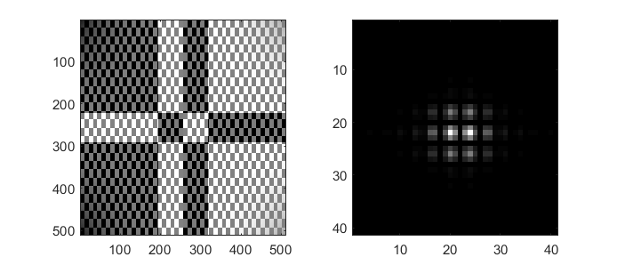
Fig. 14 A phase pattern (left) to generate a HG beam in the far-field (right). This pattern accounts for non-uniform incident illumination.

Creating a Bessel beam

A bessel-like beam can be created in the far-field of the SLM by creating a annular ring on the device. The phase of the ring can be constant for Bessel beams without angular momentum, or an azimuthal phase can be added for Bessel beams with angular momentum. To create the Bessel beam, we need a ring with a finite power and infinitely small thickness. This is difficult to achieve, so instead it is better to create a ring with a finite thickness, for this we can use the otslm.simple.aperture() function to create a ring. We can replace the regions outside the aperture with a checkerboard pattern to scatter the light to high angles. Example output is shown in Fig. 15.

pattern = otslm.simple.aperture(sz, [ 100, 110 ], 'shape', 'ring');

% Coorect for amplitude of beam
pattern = pattern .* beamCorrection;

% Finalize pattern
pattern = otslm.tools.finalize(zeros(sz), 'amplitude', pattern);

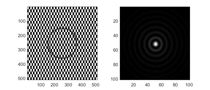
Fig. 15 A bessel-like beam generated using a finite thickness ring. A checkerboard pattern is used to scatter unwanted light away from the desired beam.

Combining patterns

There are multiple methods for combining beams. The phases can be added or multiplied or the complex amplitudes can be added or multiplied.

Adding phase patterns

Beam phase patterns can be added together at any time. This can be useful for beam steering, for example, a linear grating or a lens could be added to another pattern to shift the location in the focal plane. It is often better to add the phase patterns before calling the finalize method, since the finalize method applies the modulo to the patterns which may introduce additional artefacts if patterns are added after this operation. An example is shown in Fig. 16.

pattern = otslm.simple.lgmode(sz, 3, 2, 'radius', 50);
pattern = pattern + otslm.simple.linear(sz, 30);
pattern = otslm.tools.finalize(pattern);

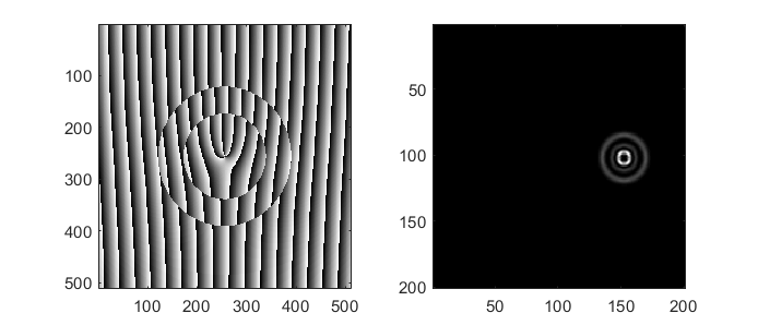
Fig. 16 A linear ramp, generated with otslm.simple.linear(), is added to a LG beam phase mask to shift the location of the LG beam in the farfield (right).

Superposition of beams

To create a superposition of different beams we can combine the complex amplitudes of the individual beams. To do this, we can use the otslm.tools.combine() function. This function provides a range of methods for combining beams, here we will demonstrate the super method. The combine function accepts additional arguments for weighted super-positions and also supports adding random phase offsets using the rsuper method. The following code demonstrates using the super method, the output is shown in Fig. 17.

pattern1 = otslm.simple.linear(sz, 30, 'angle_deg', 90);
pattern2 = otslm.simple.linear(sz, 30, 'angle_deg', 0);

pattern = otslm.tools.combine({pattern1, pattern2}, ...
    'method', 'super');

pattern = otslm.tools.finalize(pattern);

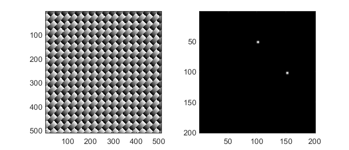
Fig. 17 Demonstration of otslm.tools.combine() for combining two linear gratings using the super-position method.

Arrays of patterns

By adding a grating, such as a 2-D sinusoidal grating, to the pattern it is possible to create arrays of similar spots. This can be a quick method for creating an array of optical traps for interacting with many similar samples. The following example shows how a sinusoid grating can be combined with a LG-mode pattern to create the output shown in Fig. 18.

lgpattern = otslm.simple.lgmode(sz, 5, 0);
grating = otslm.simple.sinusoid(sz, 50, 'type', '2dcart');

pattern = lgpattern + grating;
pattern = otslm.tools.finalize(pattern, 'amplitude', beamCorrection);

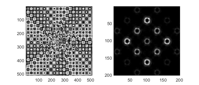
Fig. 18 An array of beams generated using a sinusoidal grating.

Selecting regions of interest

Spatial light modulators can be used for creating beams and sampling light from specific regions of beams for novel imaging applications. The toolbox provides a method to help with creating region masks for sampling different regions of the device. In this example, we show how otslm.tools.mask_regions() can be used to sample three regions of the device to create three separate beams.

The first stage is to setup three different spots. We specify the location of each spot, the radius and the pattern. We use otslm.tool.finalize() to apply amplitude corrections and apply the modulo to the patterns but we request the output remain in the range [0, 1).

loc1 = [ 170, 150 ];
radius1 = 75;
pattern1 = otslm.simple.lgmode(sz, 3, 0, 'centre', loc1);
pattern1 = pattern1 + otslm.simple.linear(sz, 20);
pattern1 = otslm.tools.finalize(pattern1, 'amplitude', beamCorrection, ...
    'colormap', 'gray');

loc2 = [ 320, 170 ];
radius2 = 35;
pattern2 = zeros(sz);

loc3 = [ 270, 300 ];
radius3 = 50;
pattern3 = otslm.simple.linear(sz, -20, 'angle_deg', 45);
pattern3 = otslm.tools.finalize(pattern3, 'amplitude', 0.4, ...
    'colormap', 'gray');

For the background we use a checkerboard pattern.

background = otslm.simple.checkerboard(sz);

To combine the patterns, we call otslm.tools.mask_regions() with the background pattern, the region patterns, their locations, radii and the mask shape (in this case a circle). We then call otslm.tools.finalize() to rescale the resulting pattern from the [0, 1) range to the [0, 2pi) range needed for the visualisation. The output is shown in Fig. 19.

pattern = otslm.tools.mask_regions(background, ...
    {pattern1, pattern2, pattern3}, {loc1, loc2, loc3}, ...
    {radius1, radius2, radius3}, 'shape', 'circle');

pattern = otslm.tools.finalize(pattern);

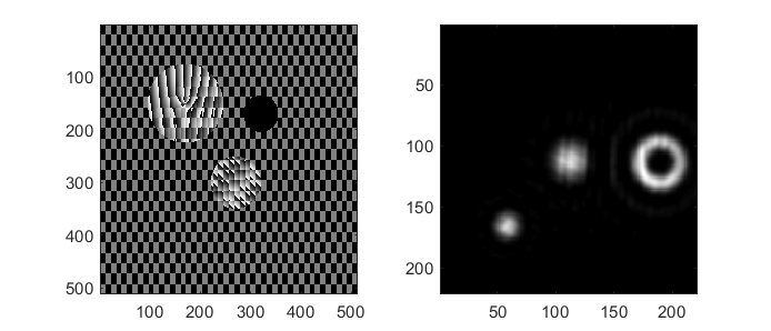
Fig. 19 Example output from otslm.tools.mask_regions() sampling three regions of interest.

Gerchberg-Saxton

The toolbox provides a number of iterative algorithms for generating patterns. One such algorithm is the Gerchberg-Saxton algorithm. This method attempts to approximate the desired light field by iteratively moving between the near-field and far-field. A more detailed overview of the algorithm can be found in the GerchbergSaxton section later in the documentation.

In OTSLM, most iterative algorithms are implemented as Matlab classes. To use the GerchbergSaxton class, we need to specify the target image. Additionally, we can specify the propagation methods to use to go between the near-field and far-field and an initial guess. In this example, we setup a propagator with the incident illumination

prop = otslm.tools.prop.FftForward.simpleProp(zeros(sz));
vismethod = @(U) prop.propagate(U .* incident);

and then create an instance of the iterator class. GerchbergSaxton also implements the adaptive-adaptive algorithm via the adaptive optional parameter, see the documentation for additional details.

target = otslm.simple.aperture(sz, sz(1)/20);
gs = otslm.iter.GerchbergSaxton(target, 'adaptive', 1.0, ...
    'vismethod', vismethod);

To run the algorithm, we simply need to call run with the number of iterations we would like to run for. The run method returns the complex amplitude pattern from the output of the last iteration. To retrieve the phase pattern, we can simply access the phase class member. This phase pattern has a range of 0 to 2pi, therefore it does not need to be passed to otslm.tools.finalize() before visualisation. Fig. 20 shows example output from this method.

gs.run(20);
pattern = gs.phase;

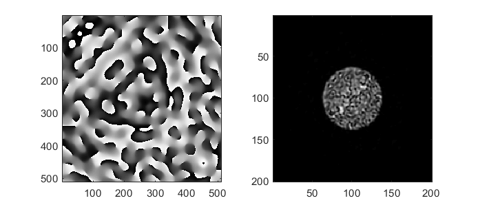
Fig. 20 Phase pattern generated using Gerchberg-Saxton (left) and the simulated far-field (right).

Creating patterns for the DMD

A digital micro-mirror device (DMD) is a binary amplitude spatial light modulator which consists of square pixels arranged in a diagonal lattice. The arrangement of pixels means that the device has a 1:2 aspect ratio. Although the device can only control the amplitude of individual pixels, it is still possible to create masks which control both the phase and amplitude of the resulting beam.

In this example, we create a LG beam using a binary amplitude pattern, following a similar approach to Lerner et al., Opt. Lett.37 (23) 4826–4828 (2012). We need to use a different size and aspect ratio for the DMD, for this example we will use a device with 512x1024 pixels.

dmdsz = [512, 1024];
aspect = 2;

To create the LG-mode pattern, we can use the otslm.simple.lgmode() function. This function has an optional argument for the aspect ratio and returns both the amplitude and phase for the pattern.

[phase, amplitude] = otslm.simple.lgmode(dmdsz, 3, 0, ...
    'aspect', aspect, 'radius', 100);

The DMD diffraction efficiency when controlling both the phase and amplitude is fairly low, so we expect there to be a significant amount of light left in the zero order. We can shift our LG beam away from the zero order light using a linear diffraction grating. There are also artefacts from the hard edges of the square (diamond) shaped pixels, to avoid these artefacts we rotate the linear grating.

phase = phase + otslm.simple.linear(dmdsz, 40, ...
    'angle_deg', 62, 'aspect', aspect);

For this example we are going to assume uniform illumination. To encode both the amplitude and phase into the amplitude-only pattern we can use the finalize function and specify that the device is a DMD and the colormap is grayscale. By default, the finalize function assumes DMDs should be rotated (packed) differently, however we want to leave our pattern unchanged for now and explicitly rotate it at a later stage, so we pass none as the rpack option.

pattern = otslm.tools.finalize(phase, 'amplitude', amplitude, ...
    'device', 'dmd', 'colormap', 'gray', 'rpack', 'none');

At this stage, the pattern is for a continuous amplitude device. To convert the continuous amplitude to a binary amplitude, we can use otslm.tools.dither(). It is possible to do this all in one step using one call to otslm.tools.finalize() but this allows additional control over the dither.

pattern = otslm.tools.dither(pattern, 0.5, 'method', 'random');

Up until now, our pattern has been in device pixel coordinates. In order to visualise what the pattern will look like in the far-field we need to re-map the device pixel coordinates to the 1:2 aspect ratio found on a physical device. For this we can use otslm.tools.finalize() again, this time with the rpack argument set to 45deg. We explicitly set no modulo and a gray-scale colour-map again, however our pattern is already binary so the output will still be zeros and ones.

patternVis = otslm.tools.finalize(pattern, ...
    'colormap', 'gray', 'rpack', '45deg', 'modulo', 'none');

The final step is to visualise the pattern. For this we create a uniform incident illumination and we call the otslm.tools.visualise() method with no phase. The output is shown in Fig. 21.

dmdincident = ones(size(patternVis));

visOutput = abs(otslm.tools.visualise([], 'amplitude', patternVis, ...
    'method', 'fft', 'padding', padding, 'incident', dmdincident)).^2;

% Zoom into the resulting pattern
visOutput = visOutput(ceil(size(visOutput, 1)/2)-50+(-40:40), ...
    ceil(size(visOutput, 2)/2 +(-40:40)));

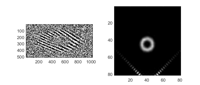
Fig. 21 Binary amplitude DMD pattern (left) generating an LG-beam beam in the far-field (right).